ch3.tensor
Ch 3. Tensor
The World as Floating-Point Numbers
Why Floating-Point Numbers?
- Deep learning models process real-world data by converting it into floating-point numbers.
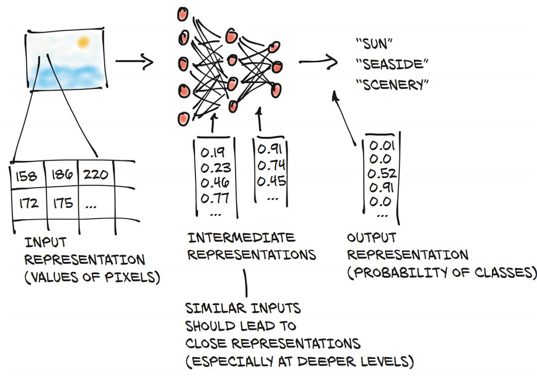
- A neural network transforms input data into an output representation through multiple intermediate steps.
- These intermediate representations capture important features, such as:
- Early layers: Detect edges, textures (e.g., fur).
- Deeper layers: Recognize structures (e.g., ears, noses, objects).
- The final representation produces probabilities for different categories (e.g., "sun," "seaside," "scenery").
Tensors: The Foundation of Data in PyTorch
- Tensors are the core data structure in PyTorch, similar to NumPy arrays but with additional capabilities.
- Definition: A generalization of vectors and matrices to an arbitrary number of dimensions (multidimensional arrays).
- Comparison with NumPy:
- PyTorch tensors seamlessly interoperate with NumPy arrays.
- They integrate well with scientific Python libraries like SciPy, Scikit-learn, and Pandas.
- Extra features:
- GPU acceleration for fast computations.
- Ability to distribute operations across multiple devices.
- Autograd support (automatically tracks computation graphs).
Understanding Tensor Dimensions
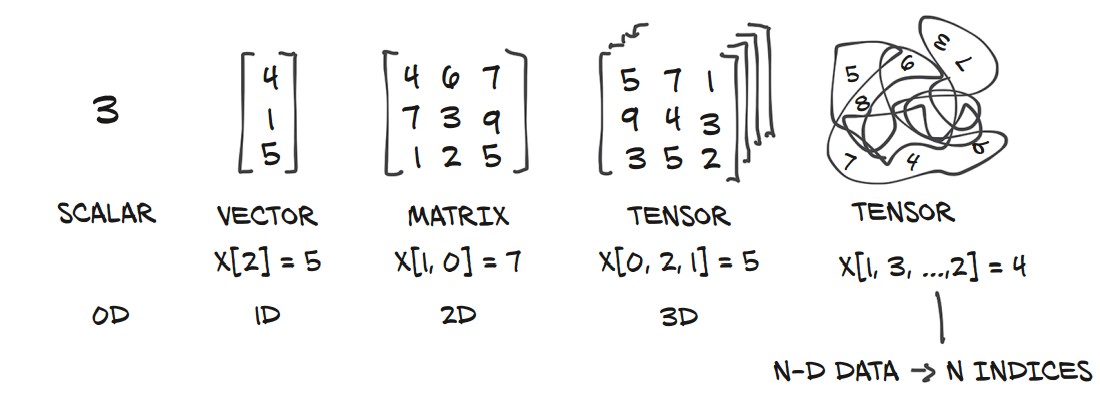
- Scalars (0D): A single number.
- Vectors (1D): A one-dimensional array.
- Matrices (2D): A two-dimensional array.
- Tensors (3D+): Multi-dimensional arrays for more complex data structures.
Example of Tensors in PyTorch:
import torch

# Scalar (0D tensor)
scalar = torch.tensor(5)

# Vector (1D tensor)
vector = torch.tensor([1, 2, 3])

# Matrix (2D tensor)
matrix = torch.tensor([[1, 2], [3, 4]])

# 3D Tensor
tensor_3d = torch.tensor([[[1, 2], [3, 4]], [[5, 6], [7, 8]]])

print(scalar.shape)    # Output: torch.Size([])
print(vector.shape)    # Output: torch.Size([3])
print(matrix.shape)    # Output: torch.Size([2, 2])
print(tensor_3d.shape) # Output: torch.Size([2, 2, 2])
Tensors: Multidimensional Arrays
What is a Tensor?
- A tensor is an array-like data structure that stores numbers and supports efficient operations.
- Similar to NumPy arrays, but with additional features like GPU acceleration and autograd support.
- Tensors enable fast and expressive data manipulation in PyTorch.
1. Creating Tensors from Python Lists
import torch

a = torch.ones(3)  # Creates a tensor of size 3 with ones
print(a)  # tensor([1., 1., 1.])

print(a[1])  # tensor(1.)
print(float(a[1]))  # Output: 1.0

a[2] = 2.0  # Modifying tensor values
print(a) # tensor([1., 1., 2.])- Unlike Python lists, PyTorch tensors store data in contiguous memory, making them much faster.
2. Understanding Tensor Storage
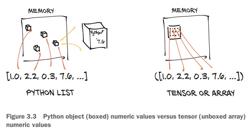
- Python lists store numbers as separate objects, requiring more memory.
- Tensors store numbers as raw C floats, making them faster and more memory-efficient.
| Python List | PyTorch Tensor |
|---|---|
| Stores numbers as individual objects in memory. | Stores numbers in contiguous memory blocks. |
| More memory overhead. | Compact and efficient storage. |
| Slower operations. | Faster computations. |
3. Creating and Indexing Tensors
Example: Representing 2D Coordinates
points = torch.tensor([[4.0, 1.0], [5.0, 3.0], [2.0, 1.0]])
print(points)
Output:
tensor([[4., 1.],
        [5., 3.],
        [2., 1.]])
Checking Tensor Shape
print(points.shape) # Output: torch.Size([3, 2])- (3, 2) → 3 rows, 2 columns (three points, each with x and y coordinates).
Initializing with zeros() or ones()
points = torch.zeros(3, 2)  # 3x2 tensor filled with zeros
print(points)
Output:
tensor([[0., 0.],
        [0., 0.],
        [0., 0.]])
Indexing Tensors in PyTorch
Basic Indexing and Slicing
-
PyTorch tensors support range indexing, similar to Python lists and NumPy arrays.
-
Example: Slicing a List
some_list = list(range(6)) print(some_list[:]) # All elements print(some_list[1:4]) # Elements 1 to 3 print(some_list[1:]) # Elements from index 1 to end print(some_list[:4]) # Elements from start to index 3 print(some_list[:-1]) # All except last element print(some_list[1:4:2]) # Step of 2 -
Example: Indexing a Tensor
import torch

points = torch.tensor([[4.0, 1.0], [5.0, 3.0], [2.0, 1.0]])

print(points[1:])      # All rows after the first
print(points[1:, :])   # All rows after first, all columns
print(points[1:, 0])   # First column of all rows after first
print(points[None])    # Adds a dimension (like unsqueeze)
Named Tensors in PyTorch
Named tensors in PyTorch provide labels for dimensions, making tensor operations more readable and reducing indexing errors. They help track different dimensions explicitly rather than relying on positional indexing.
Consider a batch of images stored as a 4D tensor:
import torch

# A single grayscale image with 3 channels (e.g., RGB)
img_t = torch.randn(3, 5, 5)  # (channels, rows, columns)

# A batch of 2 images
batch_t = torch.randn(2, 3, 5, 5)  # (batch, channels, rows, columns)
To convert an RGB image to grayscale, one simple approach is to take the mean across the channel dimension. Since channels are the third dimension from the end (-3), we can use:
img_gray_naive = img_t.mean(-3)  # Mean across the channel dimension
batch_gray_naive = batch_t.mean(-3)

print(img_gray_naive.shape)  # torch.Size([5, 5])
print(batch_gray_naive.shape)  # torch.Size([2, 5, 5])
This naive approach treats all channels equally and does not account for the different perceptual importance of colors. To get a perceptually accurate grayscale conversion, we need a weighted sum instead.
Instead of a simple mean, a weighted sum based on human visual perception is often preferred. We use the standard luminance weights:
# Weights for converting RGB to grayscale
weights = torch.tensor([0.2126, 0.7152, 0.0722])
Applying Weights via Broadcasting
PyTorch’s broadcasting allows operations between tensors of different shapes. To apply the weights, we need to reshape them to match the dimensions of img_t and batch_t.
# Reshape weights to match tensor dimensions
unsqueezed_weights = weights.unsqueeze(-1).unsqueeze(-1)  # Shape: (3, 1, 1)

# Apply weights element-wise
img_weights = img_t * unsqueezed_weights  # Shape: (3, 5, 5)
batch_weights = batch_t * unsqueezed_weights  # Shape: (2, 3, 5, 5)

# Sum across the channel dimension (-3)
img_gray_weighted = img_weights.sum(-3)
batch_gray_weighted = batch_weights.sum(-3)

print(img_gray_weighted.shape)  # torch.Size([5, 5])
print(batch_gray_weighted.shape)  # torch.Size([2, 5, 5])
Explanation of Broadcasting Steps
-
Expanding Weights:
-
weights.unsqueeze(-1).unsqueeze(-1)reshapes(3,) → (3, 1, 1), making it compatible for element-wise multiplication with tensors of shape(3, H, W). -
When calling
.unsqueeze(dim), PyTorch inserts a new dimension at indexdim, shifting all later dimensions to the right.
-
| Original Shape | unsqueeze(0) → Add at start |
unsqueeze(-1) → Add at end |
|---|---|---|
(3,) |
(1, 3) |
(3, 1) |
(3, 4) |
(1, 3, 4) |
(3, 4, 1) |
(3, 4, 5) |
(1, 3, 4, 5) |
(3, 4, 5, 1) |
-
Multiplication:
- The weighted tensor maintains the original shape but has per-channel weights applied.
-
Summation:
- The final sum across the channel dimension collapses it, producing a grayscale image.
Using einsum for Compact Operations
PyTorch’s einsum (Einstein summation notation) provides a concise way to express tensor operations, eliminating the need for explicit reshaping and summation
einsum(adapted from NumPy) specifies an indexing mini-language)
img_gray_weighted_fancy = torch.einsum('...chw,c->...hw', img_t, weights)
batch_gray_weighted_fancy = torch.einsum('...chw,c->...hw', batch_t, weights)

print(batch_gray_weighted_fancy.shape)  # torch.Size([2, 5, 5])
The Einstein summation (einsum) notation in PyTorch provides a powerful and concise way to perform complex tensor operations, such as matrix multiplications and reductions, without needing explicit loops or broadcasting.
img_gray_weighted = torch.einsum('...chw,c->...hw', img_t, weights)performs a weighted sum over the channel dimension to convert an RGB image to grayscale.
-
...(Ellipsis)- Represents any preceding batch dimensions.
- This makes the operation flexible for both single images and batches of images.
- If
img_thas shape(3, H, W), then...is empty. - If
img_thas shape(B, 3, H, W), then...corresponds toB(batch size).
-
chw(Channels, Height, Width)- The input tensor
img_thas dimensions(C, H, W)or(B, C, H, W). crefers to the color channels (e.g., RGB = 3).h, ware the height and width of the image.
- The input tensor
-
c(Weights' Dimension)weightshas shape(C,), representing a weight for each channel (R, G, B).cinchwandcincindicate that they should be multiplied element-wise.
-
-> ...hw(Output Shape)- The result must have height and width (
hw). - The channel dimension (
c) is summed out, collapsing the RGB channels into a single grayscale value per pixel.
- The result must have height and width (
For each pixel (h, w), the grayscale value is computed as:
$ \text{gray}(h, w) = R(h, w) \times 0.2126 + G(h, w) \times 0.7152 + B(h, w) \times 0.0722 $
This is effectively a dot product between the C channels of the image and the C weights.
What Happens Here?
-
...represents the batch dimensionB=2, meaning the operation applies independently to each image in the batch. -
The weighted sum is performed per pixel across the
Cchannels. -
For each image in the batch, the grayscale transformation is: $ \text{gray}_b(h, w) = R_b(h, w) \times 0.2126 + G_b(h, w) \times 0.7152 + B_b(h, w) \times 0.0722 $
-
The same logic applies, but now for multiple images in parallel.
-
Overall:
| Component | Meaning |
|---|---|
... |
Handles any batch dimension, making it flexible for both single and batched images |
chw |
Represents the input image tensor with channels (c), height (h), and width (w) |
c |
Refers to the RGB weights, which match the channel dimension |
...hw |
The output shape after summing over channels (c), leaving only height & width |
Why Use einsum Instead of Broadcasting?
Instead of using:
weights_expanded = weights.unsqueeze(-1).unsqueeze(-1)  # (3, 1, 1)
img_gray_weighted = (img_t * weights_expanded).sum(-3)
einsum('...chw,c->...hw') does the same in a single, optimized step:
- Concise & Readable: No need for explicit unsqueeze or sum operations.
- Efficient: Reduces memory overhead by avoiding intermediate tensors.
- Flexible: Works for both single images and batches.
Assigning Names to Tensor Dimensions
-
PyTorch introduced named tensors in version 1.3 (experimental).
-
Creating a named tensor:
weights_named = torch.tensor([0.2126, 0.7152, 0.0722], names=['channels']) print(weights_named.names) # ('channels',) -
Refining names for existing tensors:
img_named = img_t.refine_names(..., 'channels', 'rows', 'columns') batch_named = batch_t.refine_names(..., 'channels', 'rows', 'columns') print(img_named.shape, img_named.names) # torch.Size([3, 5, 5]) ('channels', 'rows', 'columns') -
Aligning named tensors:
weights_aligned = weights_named.align_as(img_named) print(weights_aligned.shape, weights_aligned.names) # torch.Size([3, 1, 1]) ('channels', 'rows', 'columns') -
Summing along a named dimension:
gray_named = (img_named * weights_aligned).sum('channels') print(gray_named.shape, gray_named.names) # torch.Size([5, 5]) ('rows', 'columns') -
Dropping names for compatibility:
gray_plain = gray_named.rename(None)
print(gray_plain.shape, gray_plain.names)
# torch.Size([5, 5]) (None, None)
Tensor Element Types in PyTorch
Why Use PyTorch Tensors Instead of Python Lists?
- Python numbers are objects (boxed), requiring extra memory for storage and reference counting.
- Python lists store pointers to objects rather than raw numerical data, making them inefficient.
- Python is slow for numerical operations compared to optimized compiled code (C/C++).
- PyTorch tensors are optimized, contiguous blocks of memory designed for fast numerical operations.
1. Specifying Data Types with dtype
- PyTorch tensors must store elements of the same type.
- Default:
torch.float32(32-bit floating point). - Common Data Types in PyTorch:
| Data Type | PyTorch dtype |
Description |
|---|---|---|
| 32-bit float (default) | torch.float32 or torch.float |
Standard for deep learning models. |
| 64-bit float (double) | torch.float64 or torch.double |
Higher precision but slower. |
| 16-bit float (half) | torch.float16 or torch.half |
Used on GPUs to save memory. |
| 8-bit integer (signed) | torch.int8 |
Small integer storage. |
| 8-bit integer (unsigned) | torch.uint8 |
Positive-only small integers. |
| 16-bit integer | torch.int16 or torch.short |
Medium-sized integers. |
| 32-bit integer | torch.int32 or torch.int |
General integer usage. |
| 64-bit integer | torch.int64 or torch.long |
Used for tensor indexing. |
| Boolean | torch.bool |
Stores True/False values. |
2. Creating Tensors with Specific Data Types
Using dtype in Tensor Constructors
import torch

# 32-bit float (default)
tensor_float = torch.ones(3, 3, dtype=torch.float32)

# 64-bit float (double precision)
tensor_double = torch.ones(3, 3, dtype=torch.float64)

# 16-bit integer
tensor_short = torch.tensor([[1, 2], [3, 4]], dtype=torch.short)

print(tensor_short.dtype)  # Output: torch.int16
Casting an Existing Tensor to a Different Type
# Convert to double (64-bit float)
tensor_double = tensor_float.double()

# Convert to short (16-bit integer)
tensor_short = tensor_float.short()

# Alternative method using `.to()`
tensor_double = tensor_float.to(torch.double)
tensor_short = tensor_float.to(dtype=torch.short)
Checking a Tensor’s Data Type
print(tensor_double.dtype)  # Output: torch.float64
print(tensor_short.dtype)   # Output: torch.int16
3. Data Type Considerations in Deep Learning
- Most neural networks use
float32for computations. float64(double precision) offers no practical accuracy benefit but increases memory and compute time.float16(half precision) reduces memory usage but may slightly impact accuracy.- Tensors used for indexing should be
int64(torch.long). - Boolean tensors are used for conditional checks (
True/False).
4. Automatic Type Conversion in Operations
-
When tensors of different types are used together, PyTorch automatically converts to the larger type.
-
Example:
tensor_64 = torch.rand(5, dtype=torch.float64) # 64-bit float tensor_short = tensor_64.to(torch.short) # Convert to 16-bit integer result = tensor_64 * tensor_short # Auto-converts to float64 print(result.dtype) # Output: torch.float64 -
Ensuring Computation in 32-bit Float:
tensor_32 = tensor_64.to(torch.float32) # Convert explicitly
The PyTorch Tensor API
Accessing Tensor Operations
-
PyTorch offers a rich set of tensor operations available in the
torchmodule. -
Operations can be called either as functions in
torchor as tensor methods. -
Example: Transposing a Tensor
import torch # Using torch module a = torch.ones(3, 2) a_t = torch.transpose(a, 0, 1) # Using tensor method a_t2 = a.transpose(0, 1) print(a.shape, a_t.shape, a_t2.shape) # Output: (torch.Size([3, 2]), torch.Size([2, 3]), torch.Size([2, 3]))- Both forms are equivalent and interchangeable.
Categories of Tensor Operations in PyTorch
1. Tensor Creation (torch.ones, torch.randn, etc.)
-
Functions for constructing tensors from scratch or other structures.
-
Examples:
x = torch.ones(3, 3)  # 3x3 tensor filled with ones
y = torch.zeros(2, 2)  # 2x2 tensor filled with zeros
z = torch.rand(4, 4)   # 4x4 tensor with random values in [0,1]
2. Indexing, Slicing, Joining, Mutating (torch.cat, torch.split, etc.)
-
Modify the structure or contents of tensors.
-
Examples:
t = torch.tensor([[1, 2, 3], [4, 5, 6]])

print(t[:, 1])  # Select all rows, column 1 → tensor([2, 5])

t_cat = torch.cat([t, t], dim=0)  # Concatenate along rows
print(t_cat.shape)  # Output: torch.Size([4, 3])
3. Mathematical Operations (torch.abs, torch.cos, torch.sqrt, etc.)
-
Perform numerical computations on tensors.
-
Types of math operations:
- Pointwise ops: Apply functions element-wise (e.g.,
torch.abs,torch.exp). - Reduction ops: Aggregate values (
torch.mean,torch.sum). - Comparison ops: Compare values (
torch.max,torch.eq). - Spectral ops: Operate in the frequency domain (
torch.fft,torch.hamming_window). - Linear algebra ops: Matrix and vector operations (
torch.matmul,torch.eig).
- Pointwise ops: Apply functions element-wise (e.g.,
-
Examples:
a = torch.tensor([-3.0, 4.0, -2.0])
print(torch.abs(a))  # tensor([3., 4., 2.])

b = torch.tensor([[1.0, 2.0], [3.0, 4.0]])
print(torch.mean(b))  # Output: tensor(2.5)
4. Random Sampling (torch.rand, torch.normal, etc.)
-
Generate random values from probability distributions.
-
Examples:
rand_tensor = torch.rand(3, 3)  # Uniform distribution [0, 1]
normal_tensor = torch.normal(mean=0, std=1, size=(3, 3))  # Standard normal distribution
5. Serialization (torch.save, torch.load)
-
Save and load tensors from files.
-
Example:
torch.save(a, 'tensor.pt')  # Save tensor to file
loaded_tensor = torch.load('tensor.pt')  # Load tensor from file
6. Parallelism (torch.set_num_threads)
-
Control CPU parallel execution for efficiency.
-
Example:
torch.set_num_threads(4) # Use 4 CPU threads
Tensors: Understanding Storage and Views in PyTorch
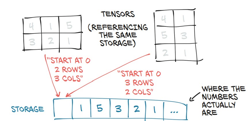
PyTorch tensors are views of storage—a contiguous block of memory that holds numerical values.
1. What is torch.Storage?
torch.Storageis a one-dimensional contiguous array storing numerical values.- A tensor is a view of this storage with indexing and dimension metadata.
- Multiple tensors can share the same storage but with different shapes and indexing rules.
2. Accessing the Underlying Storage
import torch

points = torch.tensor([[4.0, 1.0], [5.0, 3.0], [2.0, 1.0]])
print(points.storage())
Output:
 4.0
 1.0
 5.0
 3.0
 2.0
 1.0
[torch.FloatStorage of size 6]
- Although
pointsis 3×2, its storage is a 1D array of size 6. - The tensor knows how to map indices to this storage.
Manually Indexing Storage
points_storage = points.storage()
print(points_storage[0])  # 4.0
print(points_storage[1]) # 1.0- Storage is always 1D, even if the tensor is multi-dimensional.
3. Shared Storage Between Tensors
Example: Modifying Storage Affects Tensors
points_storage[0] = 2.0  # Modify storage
print(points)  # The tensor updates as well
Output:
tensor([[2., 1.],
        [5., 3.],
        [2., 1.]])
- Changing storage directly updates all tensors that reference it.
4. In-Place Tensor Operations (_ Suffix)
-
Operations ending with
_modify the tensor in-place. -
Example: Zeroing Out a Tensor In-Place
a = torch.ones(3, 2)
a.zero_()  # Modifies the tensor directly
print(a)
Output:
tensor([[0., 0.], [0., 0.], [0., 0.]]) -
Other In-Place Operations:
b = torch.rand(3, 3) b.add_(2) # Adds 2 to each element in-place b.mul_(3) # Multiplies each element by 3 in-place -
Why Use In-Place Operations?
- Saves memory by avoiding tensor copies.
- Can improve performance, especially on large tensors.
- But beware! In-place operations overwrite gradients in autograd computations.
Tensor Metadata: Size, Offset, and Stride
A tensor is a view of a storage, and three key metadata attributes define how a tensor maps to that storage:
- Size (Shape) – Number of elements in each dimension.
- Offset – Index of the first element in the storage.
- Stride – Steps to take in storage to move along each dimension.
1. Viewing Tensor Storage
Each tensor has a storage that holds its actual data as a 1D contiguous array.
import torch

points = torch.tensor([[4.0, 1.0], [5.0, 3.0], [2.0, 1.0]])
print(points.storage())
Output:
 4.0
 1.0
 5.0
 3.0
 2.0
 1.0
[torch.FloatStorage of size 6]
- The storage is 1D even though the tensor is 2D (3×2).
- The tensor maps its indices to positions in this storage.
2. Offset: Finding a Tensor's Starting Position in Storage
second_point = points[1]  # Extract the second row
print(second_point.storage_offset()) # 2- Offset = 2 because the first row (2 elements) is skipped in storage.
3. Stride: How a Tensor Maps to Storage
print(points.stride()) # Output: (2, 1)- Row stride (2): Move 2 elements forward to get to the next row.
- Column stride (1): Move 1 element forward to get to the next column.
For a tensor points[i, j], its position in storage is:
storage_index = points.storage_offset() + (i * points.stride()[0]) + (j * points.stride()[1])So points[1, 1] → offset 2 + (1 * 2) + (1 * 1) = 5, which maps to value 3.
4. Subtensors Share Storage
- Extracting a subtensor does not copy data, it just creates a new view.
- Changing the subtensor modifies the original tensor.
second_point[0] = 10.0
print(points)
Output:
tensor([[ 4.,  1.],
        [10.,  3.],
        [ 2.,  1.]])
- Solution: Clone the tensor to avoid modifying the original.
second_point = points[1].clone()5. Transposing a Tensor Without Copying
- Transpose does not reallocate storage, it just changes strides.
points_t = points.t()
print(points_t.stride()) # (1, 2)- Before:
points.stride() = (2, 1)(row-major order) - After Transpose:
points_t.stride() = (1, 2)(column-major order)
Verifying Shared Storage
print(id(points.storage()) == id(points_t.storage())) # True- The transpose operation is fast since no memory is copied.
6. Transposing Higher-Dimensional Tensors
some_t = torch.ones(3, 4, 5)
transpose_t = some_t.transpose(0, 2)
print(transpose_t.shape)  # torch.Size([5, 4, 3])
print(transpose_t.stride()) # (1, 5, 20)- Higher-dimension transposes reorder stride values instead of reallocating storage.
7. Contiguous Tensors
- A tensor is contiguous if its storage is laid out sequentially in memory.
- Transposing often makes a tensor non-contiguous.
print(points.is_contiguous())  # True
print(points_t.is_contiguous())  # False

"""
Memory layout (row-major order):
[ 1, 2, 3, 4, 5, 6 ]

Stored as: (row-first)
[[ 1, 2 ],
 [ 3, 4 ],
 [ 5, 6 ]]

After transformed

Access pattern (column-first):
[[ 1, 3, 5 ],
 [ 2, 4, 6 ]]

No longer contiguous accessing as actual memory is still
[ 1, 2, 3, 4, 5, 6 ]
"""
Making a Tensor Contiguous
To convert a non-contiguous tensor into a contiguous one:
points_t_cont = points_t.contiguous()
print(points_t_cont.stride()) # (3, 1)- A new contiguous memory block is allocated.
- The data is copied and rearranged in the correct order.
- Stride is reset to reflect the new contiguous layout.
Moving Tensors to the GPU
PyTorch tensors can be transferred from CPU to GPU for faster, parallelized computations. The device attribute determines whether a tensor is stored in system RAM (CPU) or GPU memory.
1. Creating a Tensor Directly on the GPU
Specify device='cuda' when creating a tensor:
import torch
points_gpu = torch.tensor([[4.0, 1.0], [5.0, 3.0], [2.0, 1.0]], device='cuda')
2. Moving an Existing Tensor to the GPU
Use .to(device='cuda') to transfer a CPU tensor to the GPU:
points = torch.tensor([[4.0, 1.0], [5.0, 3.0], [2.0, 1.0]])
points_gpu = points.to(device='cuda')- This returns a new tensor on the GPU while keeping the original CPU tensor intact.
- Operations on GPU tensors execute using CUDA routines.
If the machine has multiple GPUs, specify the GPU index (zero-based):
points_gpu = points.to(device='cuda:0') # Use first GPU3. Performing Operations on the GPU
Once a tensor is on the GPU, all mathematical operations are executed on the GPU:
points_gpu = 2 * points.to(device='cuda') # Multiplication occurs on the GPU- The tensor remains on the GPU after the operation.
- No CPU-GPU data transfer happens unless explicitly requested.
4. Moving a Tensor Back to the CPU
To transfer a GPU tensor back to the CPU, use:
points_cpu = points_gpu.to(device='cpu')Alternatively, use shorthand methods:
points_cpu = points_gpu.cpu()  # Move to CPU
points_gpu = points.cuda() # Move to GPU.cuda(0)moves the tensor to the first GPU (use.cuda(1),.cuda(2), etc., for other GPUs).- Using
.to(device='cpu')or.cpu()ensures that the tensor is accessible by non-GPU functions.
5. Changing Device and Data Type Together
Use .to() to move and change dtype simultaneously:
points_gpu = points.to(dtype=torch.float16, device='cuda')This converts the tensor to 16-bit floating point and moves it to the GPU in one step.
NumPy Interoperability in PyTorch
PyTorch seamlessly interoperates with NumPy by sharing memory when working on the CPU. This allows efficient conversions without copying data.
1. Converting a PyTorch Tensor to a NumPy Array
Use .numpy() to convert a PyTorch tensor to a NumPy array:
import torch

points = torch.ones(3, 4)  # Create a 3x4 tensor
points_np = points.numpy()  # Convert to NumPy array
print(points_np)
Output:
array([[1., 1., 1., 1.],
       [1., 1., 1., 1.],
       [1., 1., 1., 1.]], dtype=float32)
✅ No copy is made: The NumPy array shares the same memory as the PyTorch tensor.
✅ Changes to one affect the other:
points_np[0, 0] = 0  # Modify the NumPy array
print(points)  # The PyTorch tensor changes too!
Output:
tensor([[0., 1., 1., 1.],
        [1., 1., 1., 1.],
        [1., 1., 1., 1.]])
❗ Exception: If the tensor is on a GPU, PyTorch will first copy it to the CPU before converting:
points_gpu = torch.ones(3, 4, device='cuda')
points_np = points_gpu.cpu().numpy()  # Move to CPU before conversion
2. Converting a NumPy Array to a PyTorch Tensor
Use torch.from_numpy() to create a tensor sharing memory with a NumPy array:
import numpy as np

np_array = np.array([[1, 2], [3, 4]], dtype=np.float32)
tensor_from_np = torch.from_numpy(np_array)
print(tensor_from_np)
Output:
tensor([[1., 2.],
[3., 4.]])np_array[0, 0] = 99
print(tensor_from_np) # PyTorch tensor updates too!Output:
tensor([[99.,  2.],
        [ 3.,  4.]])
3. Handling Default Data Types
- PyTorch default dtype:
torch.float32 - NumPy default dtype:
float64 - Solution: Explicitly convert after conversion if needed:
tensor_float32 = torch.from_numpy(np_array).to(torch.float32)Generalized Tensors in PyTorch
PyTorch provides various tensor types beyond the standard dense tensors, allowing efficient computation on different hardware and specialized memory layouts.
1. PyTorch’s Tensor Dispatching System
PyTorch automatically determines the correct computation functions based on:
- Hardware type (CPU, GPU, TPU, etc.).
- Memory layout (Dense, Sparse, Quantized).
✅ Unified API: Users interact with tensors the same way, regardless of how they are implemented.
✅ Backend Dispatching: The appropriate backend is selected automatically.
2. Types of Generalized Tensors
| Tensor Type | Description |
|---|---|
| Dense (Strided) Tensor | Standard tensor (default in PyTorch), stored in contiguous memory. |
| Sparse Tensor | Stores only nonzero values, reducing memory usage for large sparse datasets. |
| Quantized Tensor | Stores data using lower-precision formats (e.g., 8-bit integers) for memory and speed efficiency. |
| TPU Tensor | Optimized for Google TPUs (work in progress). |
| Meta Tensor | Exists only for shape inference, without actual data allocation. |
3. Sparse Tensors (Efficient for Large Sparse Data)
Example: Creating a sparse tensor to store only nonzero values:
import torch

# Define indices (positions of nonzero values)
indices = torch.tensor([[0, 1, 1], [2, 0, 2]])  # Rows & columns
values = torch.tensor([3, 4, 5])  # Nonzero values

# Create a sparse tensor
sparse_tensor = torch.sparse_coo_tensor(indices, values, (3, 3))
print(sparse_tensor)
Output:
tensor(indices=tensor([[0, 1, 1],
                        [2, 0, 2]]),
       values=tensor([3, 4, 5]),
       size=(3, 3), nnz=3, layout=torch.sparse_coo)
✅ Uses less memory compared to a dense matrix with mostly zeroes.
4. Quantized Tensors (Memory-Efficient for Inference)
Quantized tensors store data using lower precision (e.g., int8 instead of float32) to reduce memory usage and computation cost.
x = torch.randn(3, 3)  # Standard tensor
x_q = torch.quantize_per_tensor(x, scale=0.1, zero_point=0, dtype=torch.qint8)
print(x_q)
✅ Used in model deployment to reduce model size and increase inference speed.
5. Moving Between Tensor Types
You can convert between different tensor types while maintaining data integrity:
dense_tensor = sparse_tensor.to_dense()  # Convert sparse → dense
sparse_again = dense_tensor.to_sparse()  # Convert dense → sparse
Serializing Tensors in PyTorch
Saving and loading tensors is crucial for preserving trained models and data. PyTorch offers built-in serialization using torch.save() and interoperability with HDF5 via the h5py library.
1. Saving and Loading Tensors with PyTorch
PyTorch uses Pickle-based serialization to store tensors, making saving and loading straightforward.
Saving a tensor to a file
import torch

points = torch.tensor([[4.0, 1.0], [5.0, 3.0], [2.0, 1.0]])

# Save tensor to a file
torch.save(points, '../data/p1ch3/ourpoints.t')
✅ Alternative method using a file descriptor
with open('../data/p1ch3/ourpoints.t', 'wb') as f:
    torch.save(points, f)
Loading the tensor back
# Load tensor from file
points = torch.load('../data/p1ch3/ourpoints.t')

# Alternatively, using a file descriptor
with open('../data/p1ch3/ourpoints.t', 'rb') as f:
    points = torch.load(f)
✅ Limitation: PyTorch’s default format is not interoperable with other frameworks. If compatibility is needed, consider HDF5.
2. Saving Tensors Interoperably with HDF5 (h5py)
HDF5 (Hierarchical Data Format v5) is widely used for storing large numerical datasets efficiently.
Installing h5py (if not installed)
conda install h5pySaving a PyTorch tensor to an HDF5 file
import h5py

# Convert PyTorch tensor to NumPy before saving
with h5py.File('../data/p1ch3/ourpoints.hdf5', 'w') as f:
    f.create_dataset('coords', data=points.numpy())  # 'coords' is a key
Loading Specific Data from HDF5 (Efficient I/O)
HDF5 allows on-disk indexing, meaning we can load only part of the dataset without reading everything into memory.
# Open the HDF5 file in read mode
with h5py.File('../data/p1ch3/ourpoints.hdf5', 'r') as f:
    dset = f['coords']  # Access dataset by key

    # Load only the last two points
    last_points_np = dset[-2:]
✅ The dataset remains on disk until accessed, improving efficiency.
✅ The result (last_points_np) behaves like a NumPy array.
Converting HDF5 Data Back to a PyTorch Tensor
last_points = torch.from_numpy(last_points_np) # Convert to PyTorch tensorOnce the HDF5 file is closed, the dataset (dset) is invalid, so all required data should be extracted before closing.