Ch 7. Telling birds from airplanes: Learning from images

Introduction to CIFAR-10 Dataset

• CIFAR-10 is a classic image classification dataset used in computer vision.
• It contains 60,000 images (32 × 32 pixels, RGB), divided into 10 classes:
  • 0: Airplane
  • 1: Automobile
  • 2: Bird
  • 3: Cat
  • 4: Deer
  • 5: Dog
  • 6: Frog
  • 7: Horse
  • 8: Ship
  • 9: Truck
• Each image is labeled with an integer corresponding to one of these classes.
• While too simple for cutting-edge deep learning research today, CIFAR-10 remains a great learning tool.
• It is often used for benchmarking image classification models and testing deep learning frameworks.
• Compared to MNIST (handwritten digit recognition), CIFAR-10 introduces color images and more complex object recognition.
• CIFAR-10 is a subclass of torch.utils.data.Dataset, making it compatible with PyTorch's data pipeline.

from torchvision import datasets

data_path = '../data-unversioned/p1ch7/'  # Directory to store the dataset

# Download the training and validation sets
cifar10 = datasets.CIFAR10(data_path, train=True, download=True)
cifar10_val = datasets.CIFAR10(data_path, train=False, download=True)

• train=True → Loads the training dataset (50,000 images).
• train=False → Loads the validation/test dataset (10,000 images).
• download=True → Downloads the dataset if not found in data_path.

type(cifar10).__mro__

(torchvision.datasets.cifar.CIFAR10,
 torchvision.datasets.vision.VisionDataset,
 torch.utils.data.dataset.Dataset,
 object)

import matplotlib.pyplot as plt
import numpy as np

# Extract a sample image and label
image, label = cifar10[0]

# Convert image to numpy and display
plt.imshow(np.array(image))
plt.title(f"Label: {label}")
plt.show()

• Converts the PIL image to a NumPy array for visualization.

Understanding the Dataset Class in PyTorch

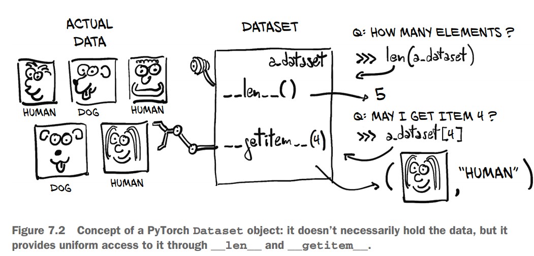
1. The Dataset Class

• torch.utils.data.Dataset is the base class for custom datasets in PyTorch.
• A dataset subclass must implement:
  • __len__() → Returns the total number of samples in the dataset.
  • __getitem__(index) → Retrieves a single sample and its corresponding label.

len(cifar10)

50000  # 50,000 training images

• Since CIFAR10 is a subclass of Dataset, it implements __len__, allowing len(cifar10) to return the total number of samples.

Accessing an Image and Label

img, label = cifar10[99]  # Accessing the 100th image
img, label

(<PIL.Image.Image image mode=RGB size=32x32 at 0x7FB383657390>, 1)

• img → A PIL (Python Imaging Library) RGB image.
• label → An integer representing the class (e.g., 1 for "automobile").

Getting the Class Name

class_names = ["airplane", "automobile", "bird", "cat", "deer",
               "dog", "frog", "horse", "ship", "truck"]
img, label, class_names[label]

(<PIL.Image.Image image mode=RGB size=32x32>, 1, 'automobile')

• The label (1) corresponds to "automobile".

Displaying the Image

import matplotlib.pyplot as plt

plt.imshow(img)
plt.title(class_names[label])  # Show the class name
plt.show()

• Displays the image using Matplotlib.
• The title shows the corresponding class ("automobile").

Dataset Transforms in PyTorch (torchvision.transforms)

Why Use Transforms?

• Many datasets (like CIFAR-10) store images as PIL images.
• Neural networks require tensors as input.
• torchvision.transforms provides built-in transformations for:
  • Converting PIL images to tensors
  • Normalizing pixel values
  • Data augmentation (random rotations, flips, crops, etc.)

from torchvision import transforms

dir(transforms)

Some common transforms:

• ToTensor() → Converts PIL images or NumPy arrays to PyTorch tensors.
• Normalize(mean, std) → Normalizes pixel values.
• RandomRotation(degrees) → Rotates images randomly.
• RandomResizedCrop(size) → Randomly crops and resizes an image.
• ToPILImage() → Converts tensors back to PIL images.

Using ToTensor() Transform

from torchvision import transforms

to_tensor = transforms.ToTensor()
img_t = to_tensor(img)  # Convert a PIL image to a tensor
img_t.shape

torch.Size([3, 32, 32])  # 3 color channels (RGB), 32x32 image

• The image is now a PyTorch tensor.
• Pixel values are scaled from [0, 255] (integers) → [0.0, 1.0] (floats).

Applying Transforms to CIFAR-10 Dataset

tensor_cifar10 = datasets.CIFAR10(
    data_path, train=True, download=False, transform=transforms.ToTensor()
)

• Now, __getitem__ returns tensors instead of PIL images.

Checking Image Type and Shape

img_t, _ = tensor_cifar10[99]
type(img_t), img_t.shape, img_t.dtype

Output:

(torch.Tensor, torch.Size([3, 32, 32]), torch.float32)

• The image is now a PyTorch tensor of type float32.
• The shape follows the convention (Channels, Height, Width) → [3, 32, 32].

Verifying Pixel Range

img_t.min(), img_t.max()

(tensor(0.), tensor(1.))  # Values are normalized to [0.0, 1.0]

Displaying the Transformed Image

import matplotlib.pyplot as plt

plt.imshow(img_t.permute(1, 2, 0))  # Convert (C, H, W) → (H, W, C) for Matplotlib
plt.show()

• The displayed image should match the original PIL image.

Normalizing Data in PyTorch (torchvision.transforms.Normalize)

Why Normalize Data?

• Ensures that each channel has zero mean and unit variance.
• Helps in faster training by keeping input values within the range where activation functions work best.
• Ensures consistent learning rates across channels.

Computing Mean and Standard Deviation for CIFAR-10

• First, stack all images into a single tensor:

imgs = torch.stack([img_t for img_t, _ in tensor_cifar10], dim=3)
imgs.shape

torch.Size([3, 32, 32, 50000])  # (Channels, Height, Width, Number of Images)

• Compute mean per channel:

imgs.view(3, -1).mean(dim=1)

tensor([0.4915, 0.4823, 0.4468])  # (Mean for Red, Green, Blue channels)

• Compute standard deviation per channel:

imgs.view(3, -1).std(dim=1)

tensor([0.2470, 0.2435, 0.2616])  # (Standard deviation for RGB channels)

Applying Normalization Using transforms.Normalize

normalize_transform = transforms.Normalize((0.4915, 0.4823, 0.4468),
                                           (0.2470, 0.2435, 0.2616))

• The first argument is mean per channel.
• The second argument is standard deviation per channel.

Chaining Transforms Using transforms.Compose

transformed_cifar10 = datasets.CIFAR10(
    data_path, train=True, download=False,
    transform=transforms.Compose([
        transforms.ToTensor(),
        transforms.Normalize((0.4915, 0.4823, 0.4468),
                             (0.2470, 0.2435, 0.2616))
    ])
)

• ToTensor() converts images to PyTorch tensors.
• Normalize() applies channel-wise normalization.

Visualizing a Normalized Image

img_t, _ = transformed_cifar10[99]
plt.imshow(img_t.permute(1, 2, 0))
plt.show()

⚠️ Issue: The image may appear black or distorted. Why?

• Normalization shifts pixel values outside the range [0,1], which Matplotlib cannot display correctly.

Undoing Normalization for Visualization

mean = torch.tensor([0.4915, 0.4823, 0.4468]).view(3, 1, 1)
std = torch.tensor([0.2470, 0.2435, 0.2616]).view(3, 1, 1)

img_t_unnorm = img_t * std + mean  # Reverse normalization
plt.imshow(img_t_unnorm.permute(1, 2, 0).clamp(0, 1))  # Ensure values stay in [0,1]
plt.show() # Now, the image will look correct!

Distinguishing birds from airplanes

Building the Dataset

Since our goal is to distinguish birds from airplanes, we need to filter CIFAR-10 to include only class 0 (airplane) and class 2 (bird) and remap the labels to be contiguous:

• Airplane → 0
• Bird → 1

Filtering and Remapping CIFAR-10

Instead of creating a subclass of torch.utils.data.Dataset, we filter and store the data in a list.

from torchvision import datasets, transforms

# Define transformation: Convert to tensor and normalize
transform = transforms.Compose([
    transforms.ToTensor(),
    transforms.Normalize((0.4915, 0.4823, 0.4468), (0.2470, 0.2435, 0.2616))
])

# Load CIFAR-10 dataset
data_path = "../data"
cifar10 = datasets.CIFAR10(data_path, train=True, download=True, transform=transform)
cifar10_val = datasets.CIFAR10(data_path, train=False, download=True, transform=transform)

# Label mapping: Airplane (0) → 0, Bird (2) → 1
label_map = {0: 0, 2: 1}
class_names = ['airplane', 'bird']

# Filter CIFAR-10 to only include airplanes and birds, and remap labels
cifar2 = [(img, label_map[label]) for img, label in cifar10 if label in [0, 2]]
cifar2_val = [(img, label_map[label]) for img, label in cifar10_val if label in [0, 2]]

# Check dataset size
print(f"Training samples: {len(cifar2)}, Validation samples: {len(cifar2_val)}")

A Fully Connected Model

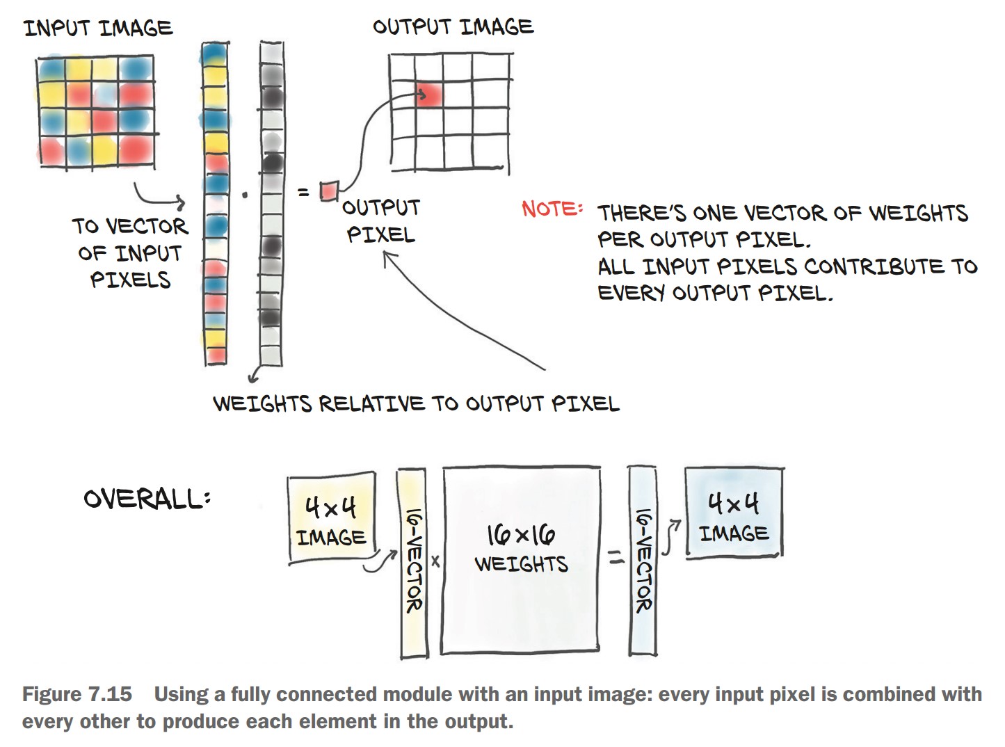
Since an image is just a set of numbers, we can flatten it into a 1D vector and treat it as a feature vector for classification.

• CIFAR-10 images have a shape of (3, 32, 32) → 3,072 pixels total (3 × 32 × 32 = 3072).
• We'll flatten the image into a 1D tensor of size 3,072 and pass it through a fully connected (dense) neural network.

Defining the Neural Network

import torch.nn as nn

# Number of output classes: 2 (Airplane or Bird)
n_out = 2

# Fully Connected Model (MLP)
model = nn.Sequential(
    nn.Linear(3072, 512),  # Input layer: 3,072 features → 512 hidden units
    nn.Tanh(),             # Activation function
    nn.Linear(512, n_out)  # Output layer: 512 hidden → 2 output classes
)

✅ Input Layer (nn.Linear(3072, 512))

• 3072 input features (flattened image pixels).
• 512 hidden units (arbitrarily chosen).

✅ Activation Function (nn.Tanh())

• Introduces non-linearity to allow learning complex relationships between pixels.
• Without activation, the model would just be a linear classifier.

✅ Output Layer (nn.Linear(512, 2))

• Reduces the hidden representation to 2 output neurons (one for each class).

🔹 Why Flatten Instead of Convolutional Layers?

• This is a simpler approach that doesn't consider spatial relationships between pixels.
• Convolutional layers (CNNs) will be introduced later to handle spatial structure more effectively.

🔹 Why Use 512 Hidden Units?

• Arbitrary choice—a balance between capacity and overfitting.
• More hidden units = higher capacity, but risk of overfitting.

🔹 Why Not More Hidden Layers?

• For this simple task, one hidden layer is often sufficient.
• Deeper networks will be used later for more complex image recognition.

Output of a Classifier

Unlike our previous regression model (predicting temperature), this task requires a categorical output:

• The image is either an airplane (0) or a bird (1).
• The output should represent probabilities, ensuring:
  • Values are in the [0, 1] range.
  • The sum of output values is exactly 1.

To achieve this, we use the softmax function. Softmax ensures:

• Each output value is between 0 and 1.
• Total sum of output values = 1 (ensuring a probability distribution).

$ \text{softmax}(x_i) = \frac{e^{x_i}}{\sum e^{x_j}} $

• Computes the exponential of each input.
• Divides each value by the sum of all exponentials.
• PyTorch provides nn.Softmax, which applies softmax along a specific dimension (e.g., across output classes).

import torch.nn as nn

softmax = nn.Softmax(dim=1)

x = torch.tensor([[1.0, 2.0, 3.0], [1.0, 2.0, 3.0]])  # Two input vectors (batch size = 2)
softmax(x)

tensor([[0.0900, 0.2447, 0.6652],
        [0.0900, 0.2447, 0.6652]])

Here, dim=1 ensures softmax is applied along the output class dimension.

We modify our neural network to include softmax at the output layer:

model = nn.Sequential(
    nn.Linear(3072, 512),
    nn.Tanh(),
    nn.Linear(512, 2),
    nn.Softmax(dim=1)  # Ensures output is a probability distribution
)

Now, the model outputs class probabilities.

img, _ = cifar2[0]  # Load a sample image
plt.imshow(img.permute(1, 2, 0))  # Display image
plt.show()

img_batch = img.view(-1).unsqueeze(0)  # Flatten image (3072,) and add batch dimension

out = model(img_batch)
print(out)

Example output

tensor([[0.4784, 0.5216]], grad_fn=<SoftmaxBackward>)

• The model returns two probabilities: one for airplane and one for bird.
• Since the model is untrained, this output is random.

Interpreting Model Predictions

We need to determine the class label from the probability output.
Use torch.max() to get the index of the highest probability:

_, index = torch.max(out, dim=1)  # Get class index
print(index)

tensor([1])  # e.g. Model predicts "bird"

A Loss for Classification

We need a better loss function than Mean Squared Error (MSE) for classification.

Why Not MSE?

• MSE focuses on exact values (0 or 1 for probabilities).
• We only care about ranking: the probability of the correct class should be higher than the incorrect one.
• MSE saturates for extreme values (very wrong predictions do not change the loss much).

Negative Log Likelihood (NLL)

• Maximizes the probability of the correct class.
• High loss if the correct class probability is low, low loss if the correct class probability is high.
• Formula:
  $ \text{NLL} = -\sum \log(p_{\text{correct class}}) $ where

$p_{\text{correct class}}$ is the probability assigned to the correct label.

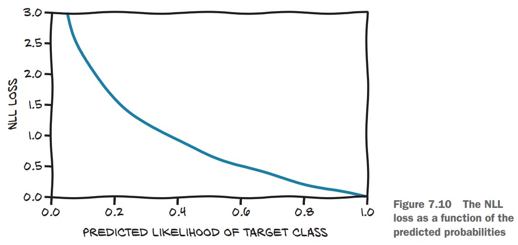
NLL Behavior

• If correct class probability = 0.99, NLL is low.
• If correct class probability = 0.01, NLL is very high.

🔹 PyTorch provides nn.NLLLoss() (Negative Log Likelihood Loss).
🔹 Important Gotcha: nn.NLLLoss() expects log probabilities as input, not raw probabilities.

To handle this, we replace nn.Softmax with nn.LogSoftmax:

import torch.nn as nn

model = nn.Sequential(
    nn.Linear(3072, 512),
    nn.Tanh(),
    nn.Linear(512, 2),
    nn.LogSoftmax(dim=1)  # Use LogSoftmax instead of Softmax
)

Then, instantiate the loss function:

loss_fn = nn.NLLLoss()

Run a sample input through the model and compute the loss:

img, label = cifar2[0]  # Load an image and its label
out = model(img.view(-1).unsqueeze(0))  # Flatten image and add batch dimension
loss_fn(out, torch.tensor([label]))  # Compute loss

tensor(0.6509, grad_fn=<NllLossBackward>)

✅ Low loss for confident correct predictions, high loss for wrong predictions.

Cross-Entropy Loss

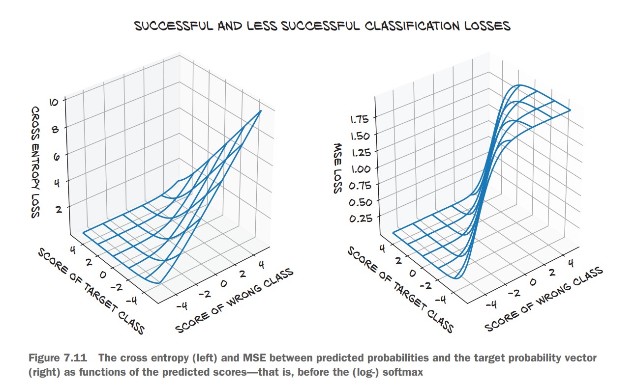
🔹 nn.CrossEntropyLoss() combines:

• Softmax (logits to probabilities)
• Negative Log Likelihood (NLL)

✅ More numerically stable than manually applying LogSoftmax + NLLLoss.

loss_fn = nn.CrossEntropyLoss()  # Preferred over NLLLoss

Training the Classifier

Training Loop

1. Define Model:

   import torch
   import torch.nn as nn
   import torch.optim as optim
   
   model = nn.Sequential(
       nn.Linear(3072, 512),
       nn.Tanh(),
       nn.Linear(512, 2),
       nn.LogSoftmax(dim=1)  # Log probabilities for classification
   )

2. Initialize Optimizer and Loss:

   learning_rate = 1e-2
   optimizer = optim.SGD(model.parameters(), lr=learning_rate)
   loss_fn = nn.NLLLoss()  # Negative Log Likelihood loss

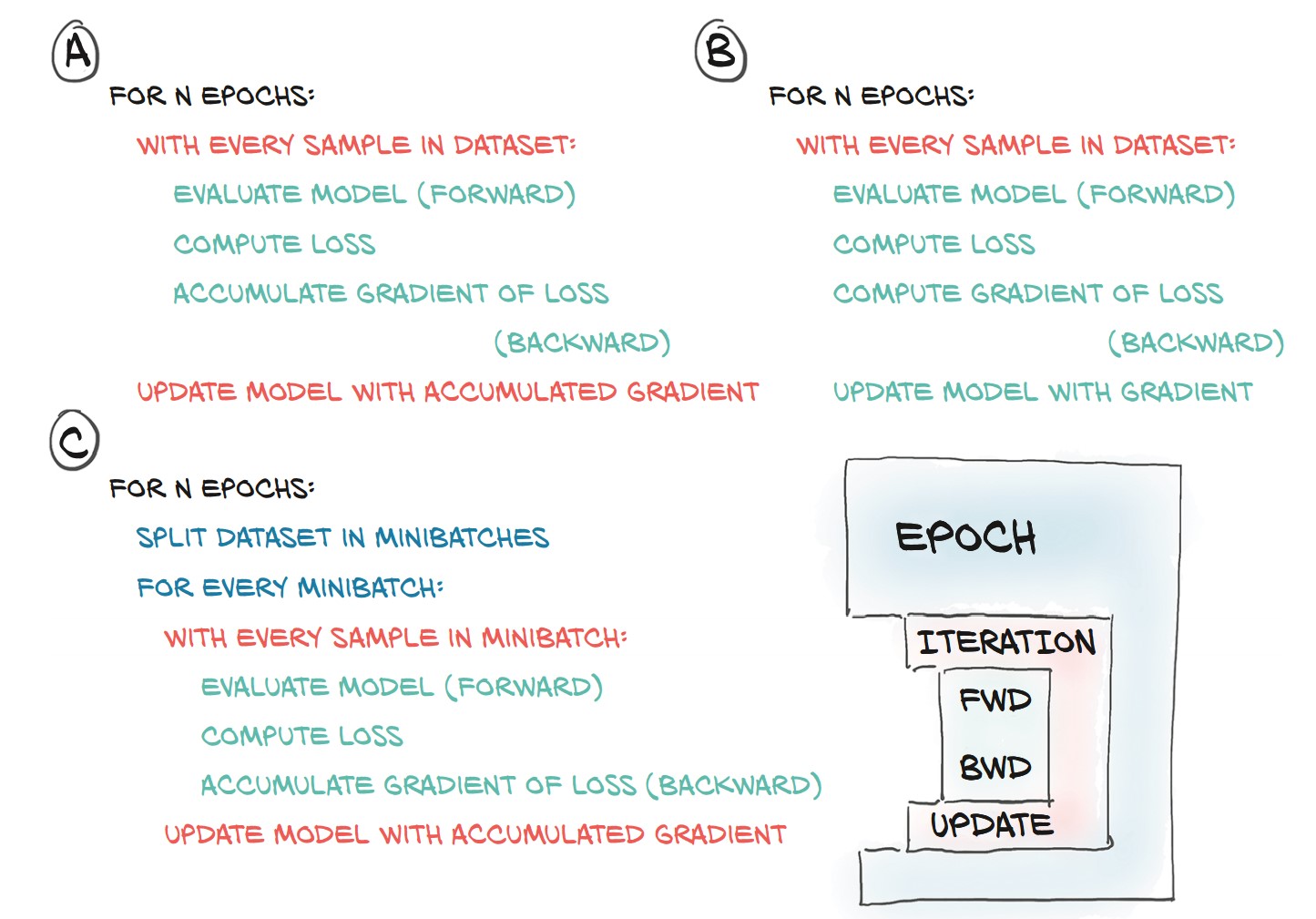
3. Training Loop Without Minibatching:

n_epochs = 100
for epoch in range(n_epochs):
    for img, label in cifar2:
        out = model(img.view(-1).unsqueeze(0))  # Flatten image
        loss = loss_fn(out, torch.tensor([label]))

        optimizer.zero_grad()
        loss.backward()
        optimizer.step()

    print(f"Epoch {epoch}, Loss: {loss.item():.6f}")

🚨 Problem:

• Processes one image at a time (inefficient).
• Loss updates based on single samples (high variance).

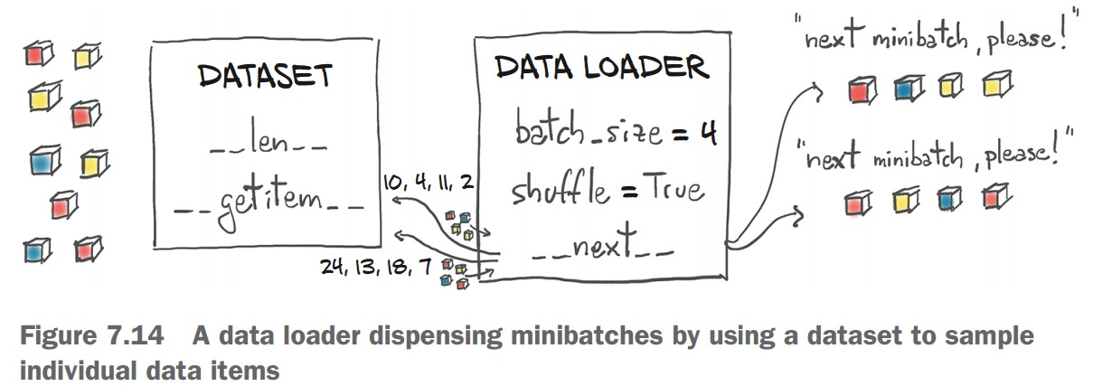
Using Minibatches with DataLoader

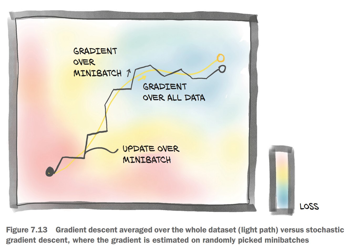
💡 Minibatches improve stability & efficiency in training.

1. Create DataLoader:

   from torch.utils.data import DataLoader
   
   train_loader = DataLoader(cifar2, batch_size=64, shuffle=True)

2. Update Training Loop to Use Minibatches:

   for epoch in range(n_epochs):
       for imgs, labels in train_loader:
           batch_size = imgs.shape[0]
           outputs = model(imgs.view(batch_size, -1))  # Flatten images
           loss = loss_fn(outputs, labels)
   
           optimizer.zero_grad()
           loss.backward()
           optimizer.step()
   
       print(f"Epoch {epoch}, Loss: {loss.item():.6f}")

Evaluating Accuracy on Validation Set

1. Create Validation DataLoader:

   val_loader = DataLoader(cifar2_val, batch_size=64, shuffle=False)

2. Compute Accuracy:

   correct = 0
   total = 0
   
   with torch.no_grad():  # Disable gradient computation
       for imgs, labels in val_loader:
           batch_size = imgs.shape[0]
           outputs = model(imgs.view(batch_size, -1))
           _, predicted = torch.max(outputs, dim=1)  # Get predicted class
   
           total += labels.shape[0]
           correct += int((predicted == labels).sum())
   
   print(f"Accuracy: {correct / total:.4f}")

   Accuracy: 0.7940
   

🎯 79.4% accuracy on validation—better than random, but not perfect.

Improving the Model

Increasing Model Depth

model = nn.Sequential(
    nn.Linear(3072, 1024),
    nn.Tanh(),
    nn.Linear(1024, 512),
    nn.Tanh(),
    nn.Linear(512, 128),
    nn.Tanh(),
    nn.Linear(128, 2),
    nn.LogSoftmax(dim=1)
)

• Accuracy improved slightly (80.2%).
• Overfitting: Training accuracy (99.8%) much higher than validation.

Alternative Loss Function: CrossEntropyLoss

💡 Combines LogSoftmax + NLLLoss automatically

model = nn.Sequential(
    nn.Linear(3072, 1024),
    nn.Tanh(),
    nn.Linear(1024, 512),
    nn.Tanh(),
    nn.Linear(512, 128),
    nn.Tanh(),
    nn.Linear(128, 2)
)

loss_fn = nn.CrossEntropyLoss()  # No need for LogSoftmax in the model

📌 Accuracy remains the same but simplifies implementation.

Key Observations

🔹 Overfitting:

• Training accuracy 99.8%, validation accuracy 80.2% → model memorizing data.

🔹 Model Size:

• First Model: 1.5M parameters
• Larger Model: 3.7M parameters
• Fully connected models scale poorly with image size.

The Limits of Fully Connected Networks for Image Classification

Using a fully connected network to classify images has severe limitations due to how it processes pixel data.

1. Why Fully Connected Networks Struggle with Images

🔹 Lack of Spatial Awareness

• The model treats each pixel independently, ignoring neighboring pixel relationships.
• The image is flattened into a 1D vector, removing spatial structure.

🔹 No Translation Invariance

• A fully connected network memorizes specific pixel locations.
• If an object (e.g., airplane) shifts position in the image, the model struggles to recognize it.

🔹 Large Number of Parameters

• Every pixel connects to every other pixel → huge number of weights.
• Scaling up to larger images (e.g., 1024×1024) becomes infeasible.

🔹 Overfitting Instead of Generalization

• The model memorizes training examples rather than learning meaningful patterns.
• Requires data augmentation (e.g., random translations) to help, but this increases computational cost.

2. Example: Why Translation Invariance Matters

• A fully connected network learns that:

  • Pixel (0,1) is dark → airplane feature
  • Pixel (1,1) is dark → airplane feature
  • …and so on.

• If the airplane shifts by 4 pixels, the entire learned relationship becomes useless!

• The model must relearn everything for every possible translation.

• This is inefficient and unnecessary because humans can recognize an airplane anywhere in the image.