ch4.scaling_with_the_compute_layer
Ch 4. Scaling with the compute layer
Intro
What are the most fundamental building blocks of data science projects?
- Data
- All data science and machine learning work begins with data—small or large.
- Compute
- Data is processed using computations (models, transformations, scoring, etc.).
- Where and how to run workflow steps (i.e., tasks).
- Especially relevant when tasks are too resource-intensive for a laptop or when using
foreachto spawn many parallel tasks.
These two components—data and compute—form the foundation of the data science infrastructure stack (as shown in Figure 4.1).
Why move beyond personal workstations?
- Example issues with local execution:
- Step needs 64 GB of memory, exceeding laptop limits.
- Workflow has a
foreachthat spawns 100+ parallel tasks, which a single workstation can’t handle efficiently.
- Solution:
- Use a cloud-based compute layer to scale beyond local limits.
What options are available for implementing a compute layer?
- There are many compute layer implementations, depending on:
- Use case
- Workload
- Budget
- Performance and availability requirements
- One recommended easy option:
- AWS Batch—a managed cloud compute service, used with Metaflow.
Why does the compute layer matter?
-
It allows projects to:
- Scale to more data
- Run more demanding computations
- Improve performance and responsiveness
-
Goal:
- Enable data scientists to tackle any business problem without infrastructure bottlenecks.
Why is understanding scalability important?
- Helps you:
- Select the right tools and compute strategies.
- Balance speed, cost, and reliability.
- Leads to smarter technical decisions and efficient workflows.
What about task failures in the compute layer?
- Running code in cloud environments introduces new failure modes.
- To maintain productivity:
- Handle errors automatically where possible.
- Provide tools for painless debugging when issues occur.
- These topics are addressed later in the chapter.
Scalability across the stack
What is scalability in the context of data science systems?
Scalability is not the same as performance, although the terms are often used interchangeably. Here's a refined definition and breakdown:
Definition of scalability
Scalability is the property of a system to handle a growing amount of work by adding resources.
Key takeaways:
- Scalability ≠ optimization — it’s about handling growth, not maximizing performance for fixed tasks.
- Requires the capacity to do more work, like handling more data or training more models.
- Involves efficiently using additional resources (e.g., more CPUs, memory, or machines).
How is scalability different from performance?
- Performance = how well the system handles a fixed task (speed, quality, efficiency).
- Scalability = how the system adapts to increased workload via added resources.
- Both are important but independent concerns.
Scalability types across the infrastructure stack
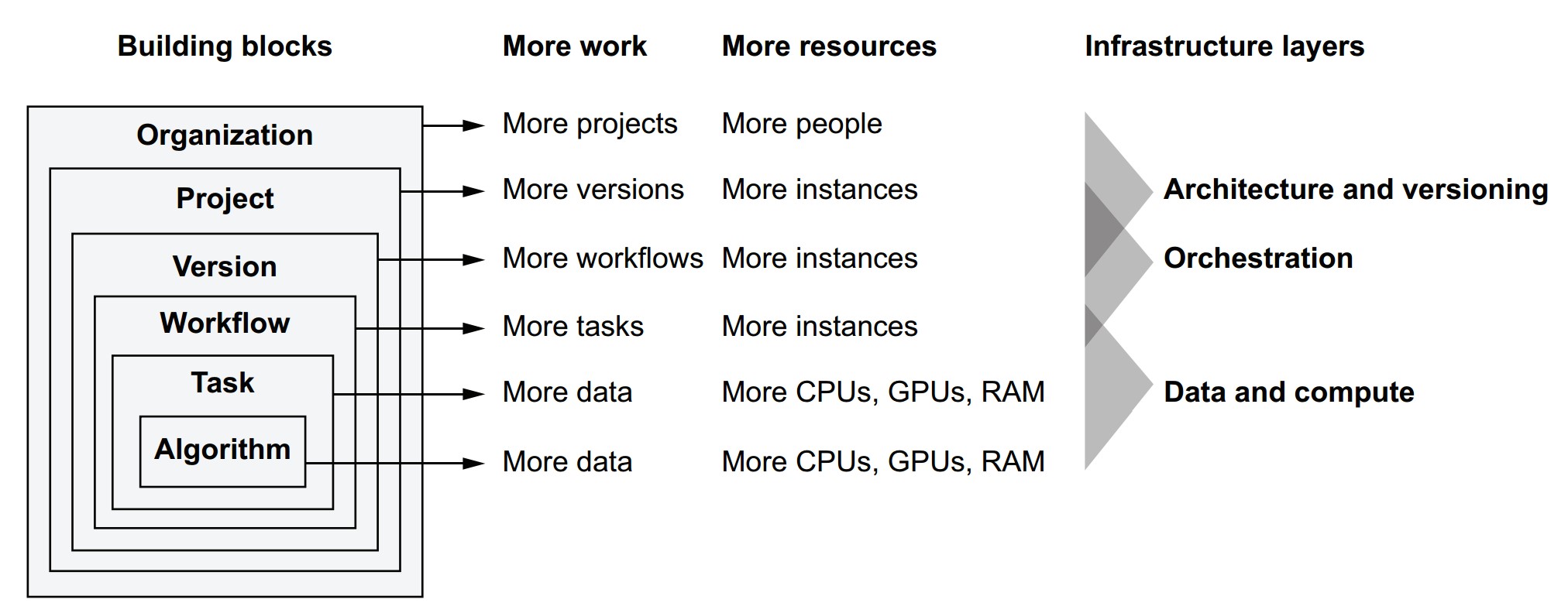
Metaflow’s stack shows how scalability applies to various components:
| Building Block | Scales With More Work | Scales By Adding | Managed By |
|---|---|---|---|
| Algorithm | More data, more complex models | More CPUs, GPUs, RAM | ML Libraries (e.g., Scikit-Learn, TensorFlow) |
| Task | Compute-bound operations | More system resources | OS Process, Code |
| Workflow | Number of concurrent tasks | More compute instances | Metaflow Runtime |
| Version | Variations in model/data | Workflow orchestrator + compute | Scheduler (e.g., Argo, AWS Step Functions) |
| Project | Parallel R&D efforts | Isolated workflows, infra per team | Namespacing, Versioning Tools |
| Organization | More people, more teams | Well-designed, modular infrastructure | Org-wide tooling and governance |
The four Vs of data science infrastructure and how they relate to scalability
- Volume – Scale to handle many projects and workflows.
- Velocity – Fast iteration: quick experiments and prototyping (i.e., performance).
- Validity – Ensures results are reliable and reproducible even as scale increases.
- Variety – Supports many models, data types, and workflows.
What does scalability really mean for a data science org?
- Compute scalability: Use more machines/cores to process more data or train more models.
- People scalability: Enable more users to experiment, collaborate, and manage independent workflows.
- Workflow scalability: Run many versions and tasks in parallel.
- Infrastructure scalability: Orchestrate many workflows without conflict or resource contention.
- Scalability is not just a technical metric—it is foundational to supporting growth in experimentation, innovation, and collaboration.
- Metaflow is designed to support scalability at every level, from algorithm to team-level operations.
Why isn’t experimentation easier in most organizations?
- Historically, compute was scarce, so access had to be carefully coordinated.
- Communication overhead increases with team size—scales quadratically with N people.
- Legacy infrastructure models (e.g., mainframes, static clusters) required centralized control, which restricts autonomy and slows experimentation.
- To support innovation, data science teams need freedom to experiment without being bottlenecked by compute limitations or coordination overhead.
How did compute access evolve?
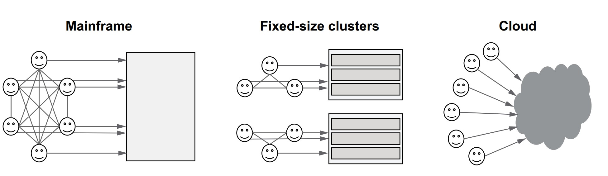
| Era | Model | Characteristics |
|---|---|---|
| 1960s | Mainframe | One shared computer; strict coordination |
| 2000s | On-prem datacenter | Dedicated clusters per team; provisioning delays |
| Today | Cloud infrastructure | Elastic compute capacity; minimal coordination |
- Today’s cloud model offers the illusion of unlimited compute:
- Access can be democratized.
- Experimentation can scale with minimal human coordination.
How does infrastructure reduce coordination overhead?
- Let the system, not humans, control access to compute.
- Use isolation to prevent workloads from interfering with one another.
- Shift from manual resource planning to on-demand, automated resource allocation.
Key benefits of minimizing coordination
- More teams can work in parallel.
- Individuals can run large-scale experiments without needing prior approval.
- Failures are isolated, not system-wide.
- Data scientists gain autonomy, reducing dependency on ML engineers or DevOps.
Practical takeaway: minimize interference to scale experimentation
Scalability tip: Minimizing interference among workloads through isolation is an excellent way to reduce the need for coordination. The less coordination is needed, the more scalable the system becomes.
Isolation tools include:
-
Containers (e.g., Docker, Kubernetes)
-
Namespaces for environment isolation
-
Versioning of code, data, and models
-
Dependency management for per-run control
-
Cloud infrastructure + good design = scalable experimentation.
-
Enables a cultural shift where data scientists can:
- Prototype independently
- Deploy at scale
- Own more of the lifecycle
-
Builds a foundation for scaling teams, projects, and workflows without bottlenecks.
The compute layer
How does the compute layer fit into the data science infrastructure stack?
The compute layer is responsible for executing individual tasks of a workflow, regardless of what the task does or why it's being executed. Its main job is to find resources and run the task.
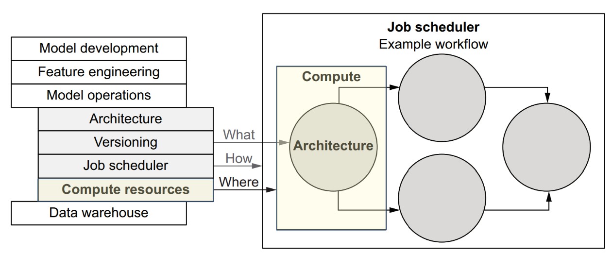
- Workflows define the logic (what to compute).
- Tasks are the executable units within workflows.
- Compute layer is responsible for running each task on an appropriate resource.
- Job scheduler/orchestrator decides when tasks run and in what order
Responsibilities of the compute layer
It provides a simple but powerful interface:
- Accept a task and its resource requirements (e.g., CPU, RAM).
- Execute the task when resources become available.
- Allow querying of task status (e.g., running, failed, succeeded).
Real-world requirements for a robust compute layer
-
Massive concurrency
- Must manage hundreds of thousands or millions of tasks.
-
Elastic hardware pool
- Computers (instances) must be added/removed without downtime.
-
Efficient task placement
- Match task resource needs to available machines.
- Complex problems: see Bin Packing and Knapsack Problem in algorithm theory.
-
Fault tolerance
- Any machine can fail.
- Tasks may behave badly or crash.
- The system must remain resilient and available under all conditions.
Then vs. now: how cloud changed compute
| Before (HPC & on-prem) | Now (Cloud) |
|---|---|
| Specialized, expensive systems | Elastic, on-demand infrastructure |
| Long provisioning times | Instant provisioning via API or UI |
| Brittle, team-managed setups | Abstracted and robust services (e.g., AWS Batch, ECS, Kubernetes) |
| Costly maintenance | Pay-as-you-go, scale when needed |
Why cloud doesn't solve everything (yet)
- The cloud provides primitive building blocks:
- You still need to build or adopt a task management system on top.
- Different compute layers (e.g., GPUs, TPUs, large memory machines) may be required depending on workload.
- Systems differ in:
- Latency
- Throughput
- Cost-efficiency
- Fault tolerance
- Scalability limits
Hence, no one-size-fits-all compute layer.
Implications for data science infrastructure
-
The infrastructure must abstract over multiple compute options, from:
- Laptops → Cloud VMs
- CPUs → GPUs → Specialized accelerators
-
All compute layers should:
- Implement a common interface
- Integrate smoothly with the workflow orchestration layer
- Be easy to swap or extend based on workload type
-
The compute layer does not need to understand workflows, just individual tasks.
-
Data scientists define the logic, goals, and resource requirements; the infrastructure handles the rest.
-
A flexible compute layer is a cornerstone of scalable and autonomous data science systems.
containers + compute layer = safe, scalable batch processing
- Batch processing defines the execution model.
- Containers provide safe, portable execution environments.
- The compute layer:
- Distributes tasks efficiently
- Scales elastically to meet demand
- Isolates workloads to boost reliability and productivity
What is batch processing with containers, and how does it support scalable compute?
Batch processing is the foundation of modern data science compute systems. Each task in a workflow is treated as a batch job: it starts, runs some code, produces output, and terminates. Containers enable this model to scale safely and reliably.
What defines a batch job?
- A batch job = user-defined code + its dependencies
- In Metaflow, each step (like
train_svm) becomes a batch job. - The compute layer:
- Executes each batch job
- Manages job resources
- Returns status/results back to the scheduler
Example step as a batch job:
@step
def train_svm(self):
    from sklearn import svm
    self.model = svm.SVC(kernel='poly')
    self.model.fit(self.train_data, self.train_labels)
    self.next(self.choose_model)
Why do we need containers?
- Code may require external dependencies (e.g.,
sklearn) not present in base environments. - A container packages:
- User code
- Dependencies
- Runtime environment
Benefits:
- Isolation: Prevents resource conflicts and interference.
- Portability: Code runs the same everywhere.
- Safety: Even buggy/malicious tasks can’t affect others.
Productivity tip: Containers allow users to run experiments freely without fear of breaking shared systems.
Execution environment
- A computer node contains:
- CPU, RAM, Disk, optional GPUs
- Operating System (e.g., Linux)
- One or more containers
- Each container runs user code + dependencies in isolation
Container format
- Most common: Docker
- Manually building containers for every iteration = impractical
- Good infrastructure (e.g., Metaflow) handles containerization automatically behind the scenes
How does a scalable compute layer work?
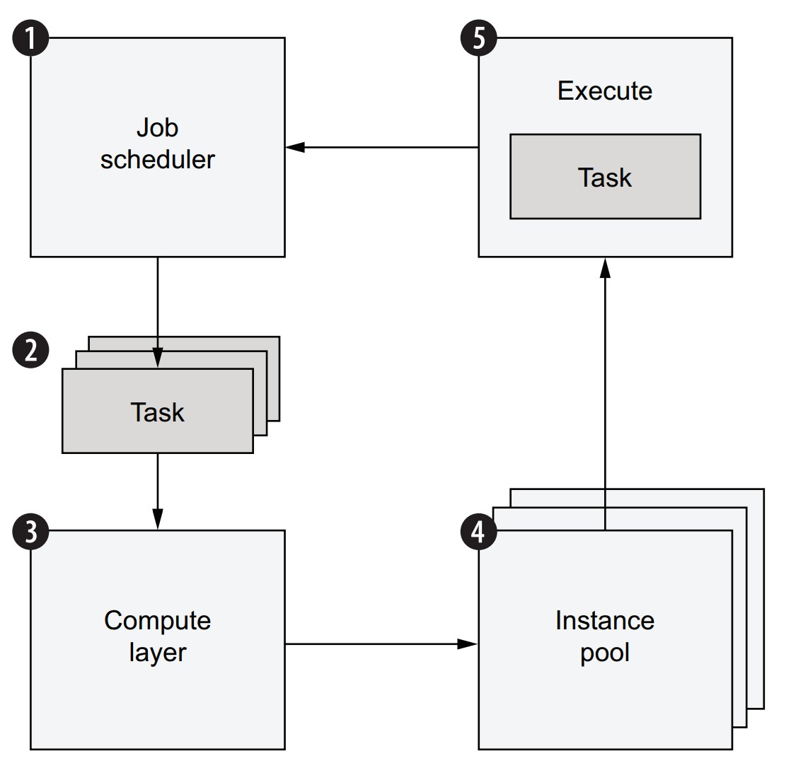
Workflow execution lifecycle:
- A job scheduler begins executing a workflow.
- Each step yields one or more tasks, submitted to the compute layer.
- Compute layer:
- Maintains a task queue
- Finds available instances to execute tasks
- If not enough resources:
- New instances are provisioned automatically
- Tasks are run in containers on available instances
- Scheduler is notified when tasks complete → moves to next step
Internal architecture of the compute layer
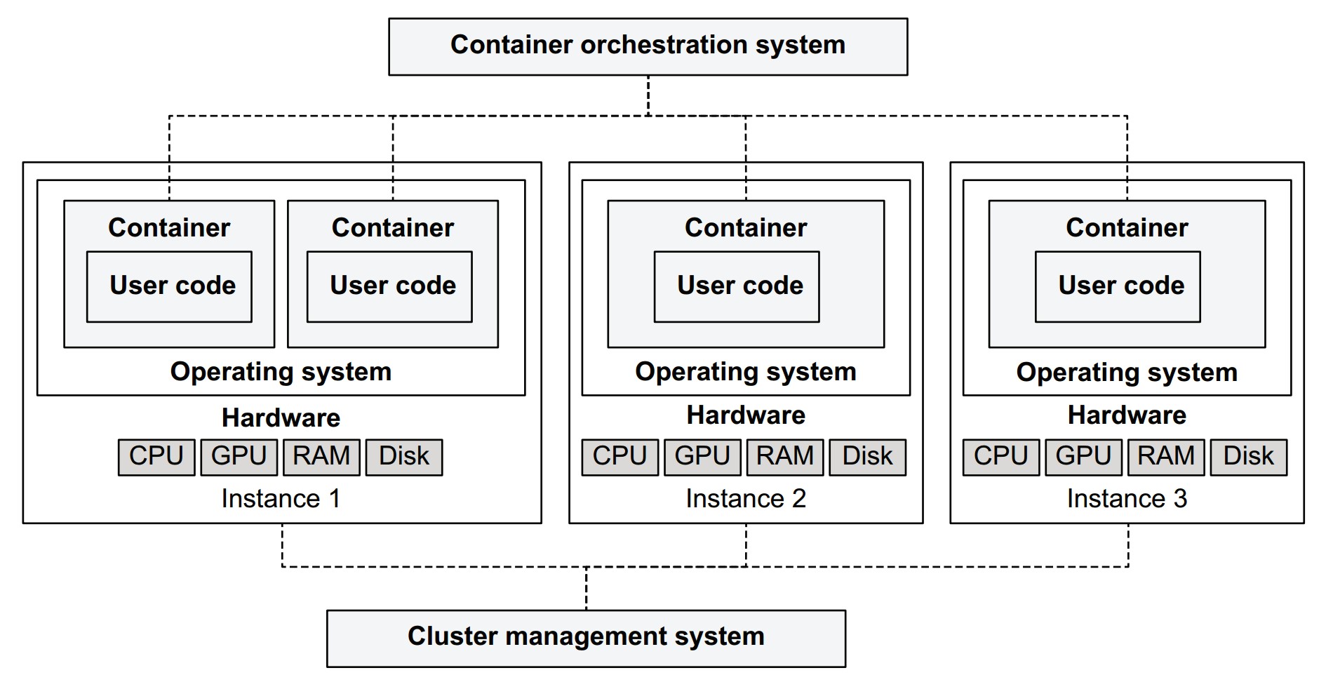
- Instance Pool:
- Computers running containers (varied CPU, GPU, RAM specs)
- Cluster Management System:
- Adds/removes instances
- Handles scaling, health checks
- Container Orchestration System:
- Maintains task queue
- Schedules tasks on suitable instances
- Matches tasks with resource requirements
Why not build this yourself?
- Compute layers are complex: hard to build reliably and efficiently.
- Use existing systems:
- Open source (e.g., Kubernetes, Apache Mesos)
- Managed cloud services (e.g., AWS Batch, GCP Cloud Run, Azure Container Apps)
Miscellaneous Notes
- Metaflow abstracts container and resource management away from users.
- Users only declare:
- The code they want to run
- The dependencies they need
- The resources (e.g., CPUs, memory) their tasks require
Scalability, safety, and flexibility are handled by the infrastructure behind the scenes.
Batch processing v.s. stream processing
- Batch processing and stream processing are two fundamental paradigms for data processing. Each serves different needs and use cases.
- Batch and stream processing are complementary, not mutually exclusive.
- Batch processing is the default and simplest starting point for most ML workflows.
- Stream processing adds value when latency is critical.
- Metaflow and similar systems are designed around batch processing.
- Stream-based integration can be layered on top or alongside using external tools.
Batch Processing
- Definition: Handles discrete, bounded units of data.
- Example: Load a dataset → process it → write results → job ends.
- Execution frequency: Typically hourly, daily, or on-demand.
- Used in:
- Machine learning training pipelines
- Data transformations and ETL
- Analytics and reporting
Pros:
- Easier to reason about
- Easier to test and debug
- Easier to scale (especially with containers and workflows)
- Fits naturally into ML workflows (e.g., Metaflow, Airflow)
Stream Processing
- Definition: Processes a continuous, unbounded stream of data in near real-time.
- Example: Clickstream analysis, fraud detection, alerting systems.
- Latency: Seconds to minutes
- Frameworks:
- Apache Kafka
- Apache Flink
- Apache Beam
- Cloud services: AWS Kinesis, Google Dataflow
Pros:
- Enables low-latency and near real-time applications
- Ideal for event-driven systems
Can you combine both?
Yes. In modern systems, hybrid architectures are common:
- Use batch processing for:
- Heavy lifting (e.g., model training, aggregation)
- Simpler system design
- Use stream processing for:
- Real-time updates (e.g., recommendations, fraud alerts)
Example: Netflix uses batch processing for model training and stream processing to keep some components updated in near real time.
When to start with batch vs. stream?
| Start with batch if... | Consider stream if... |
|---|---|
| You want simplicity and faster iteration | You need real-time updates |
| Your data is naturally bounded or historical | Your data arrives continuously |
| Your ML use case doesn’t require real-time feedback | You’re building an alerting or monitoring system |
Examples of compute layers
Different compute layers are suited to different workloads. Supporting multiple compute layers in your infrastructure enables flexibility and scalability across a range of data science projects.
Why use multiple compute layers?
- No single system is perfect for all types of workloads.
- Different projects vary in:
- Data volume
- Compute intensity
- Hardware needs
- Latency expectations
Rule of thumb:
Use one general-purpose layer (e.g., AWS Batch or Kubernetes) and a low-latency layer (e.g., local processes) for prototyping. Add others as needed.
- Pretending that one system can do it all leads to friction.
- The right balance = provide flexibility under the hood + simplicity at the surface.
- Managed services reduce operational burden but may limit flexibility.
- Open-source systems offer control but require expertise to operate reliably.
Example projects and their compute layer mix
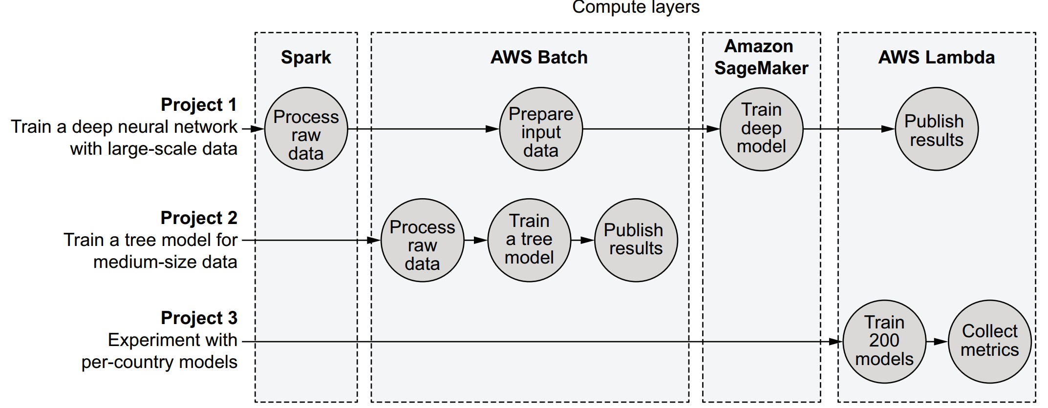
| Project | Description | Compute Layers Used |
|---|---|---|
| Project 1 | Large dataset (100 GB) + deep learning | Spark → AWS Batch → SageMaker → AWS Lambda |
| Project 2 | Medium-scale decision tree (50 GB) | AWS Batch |
| Project 3 | Small models for multiple countries | AWS Lambda |
Key compute layer options
1. Kubernetes (K8s)
- Open-source container orchestration
- Highly flexible, complex to manage
- Good for custom, large-scale environments
🔹 Use case: Custom microservices, long-running services, advanced pipelines
2. AWS Batch
- Simplified batch job execution on AWS
- Manages queues, instance pools, and containers
🔹 Use case: General-purpose workflows, medium to large batch jobs
3. AWS Lambda
- Function-as-a-Service (FaaS)
- Lightweight, fast-starting tasks; limited runtime and memory
🔹 Use case: Prototyping, small-scale parallel tasks, event-driven steps
4. Apache Spark
- Open-source distributed data processing
- Uses RDDs, DataFrames, and SQL-like APIs
🔹 Use case: Big data transformations, ETL, scalable aggregations
5. Distributed Training Platforms (e.g., SageMaker, Horovod)
- Optimized for training large neural networks
- Often GPU-backed or custom hardware
🔹 Use case: Deep learning at scale
6. Local Processes / Cloud Workstations
- Personal development machines or cloud IDEs
- Low-latency but not scalable
🔹 Use case: Fast prototyping, development iteration
Features to evaluate when choosing a compute layer
| Feature | Description |
|---|---|
| Workload support | General vs. specialized workloads |
| Latency | How quickly tasks start (important for prototyping) |
| Workload management | Queuing, task preemption, overload behavior |
| Cost-efficiency | Utilization, billing granularity |
| Operational complexity | Ease of deployment, debugging, maintenance |
Summary of system characteristics
| Feature | Local | Kubernetes | Batch | Lambda | Spark | Distributed training |
|---|---|---|---|---|---|---|
| Excels at general-purpose compute | ⭐⭐ | ⭐⭐⭐ | ⭐⭐⭐ | ⭐⭐ | ⭐⭐ | ⭐ |
| Excels at data processing | ⭐⭐ | ⭐⭐ | ⭐⭐ | ⭐ | ⭐⭐⭐ | ⭐⭐ |
| Excels at model training | ⭐⭐ | ⭐⭐ | ⭐⭐ | ⭐ | ⭐⭐ | ⭐⭐⭐ |
| Tasks start quickly | ⭐⭐⭐ | ⭐⭐ | ⭐⭐ | ⭐⭐⭐ | ⭐⭐ | ⭐ |
| Can queue a large number of pending tasks | ⭐ | ⭐⭐ | ⭐⭐⭐ | ⭐⭐⭐ | ⭐⭐⭐ | ⭐⭐ |
| Inexpensive | ⭐ | ⭐⭐ | ⭐⭐⭐ | ⭐⭐⭐ | ⭐⭐⭐ | ⭐⭐ |
| Easy to deploy and operate | ⭐⭐ | ⭐ | ⭐⭐ | ⭐⭐⭐ | ⭐ | ⭐ |
| Extensibility | ⭐⭐⭐ | ⭐⭐⭐ | ⭐⭐ | ⭐ | ⭐⭐ | ⭐⭐ |
- Choose compute layers based on workload characteristics and organizational needs.
- Keep the user experience unified: abstract away the differences between compute layers.
- Metaflow is an example of a tool that integrates multiple compute layers under one Pythonic interface
The compute layer in Metaflow
How does Metaflow support pluggable compute layers?
Metaflow tasks are isolated units of computation that can be executed on various compute layers (e.g., local, AWS Batch, Kubernetes). A single workflow can mix and match compute layers depending on task needs.
How are Metaflow tasks executed locally?
from metaflow import FlowSpec, step
import os

global_value = 5

class ProcessDemoFlow(FlowSpec):
    @step
    def start(self):
        global global_value
        global_value = 9
        print('process ID is', os.getpid())
        print('global_value is', global_value)
        self.next(self.end)

    @step
    def end(self):
        print('process ID is', os.getpid())
        print('global_value is', global_value)

if __name__ == '__main__':
ProcessDemoFlow()global_valueappears reset inend, showing each task runs in its own process.- Output:
startstep: global_value = 9endstep: global_value = 5
🔹 Use self.global_value to persist values between steps.
Key assumptions in Metaflow's compute layer design
- Different projects have diverse compute needs—some need high memory, others need GPUs, etc.
- Individual workflows have tasks with varying requirements—IO-heavy steps vs. quick control tasks.
- Needs change over time—start with local prototyping, then scale with cloud resources.
What is AWS Batch, and how does it integrate with Metaflow?
AWS Batch is a job queue system for running tasks in containers on the cloud.
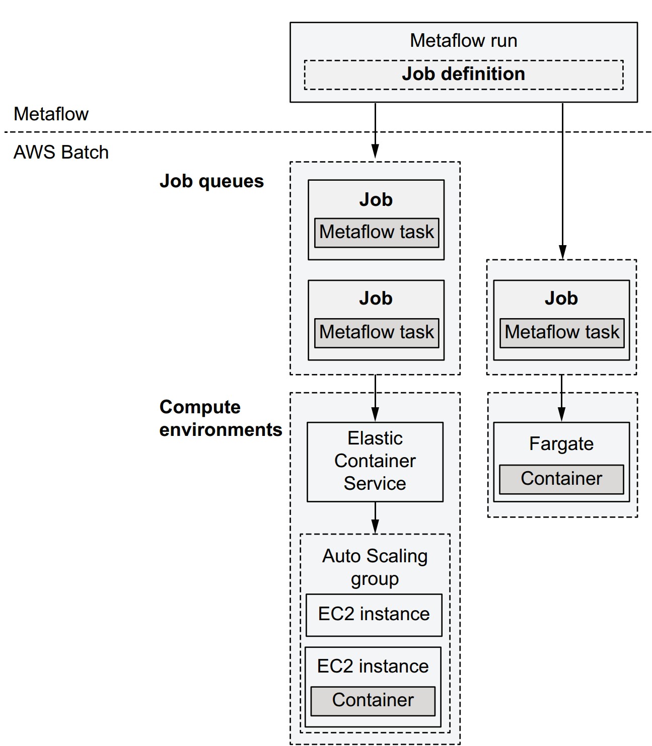
- Job Definition: Configures execution (CPU, memory, env variables).
- Job: Single computation unit (mapped 1:1 with a Metaflow task).
- Job Queue: Holds submitted jobs until resources are available.
- Compute Environment: Pool of instances (e.g., EC2 or Fargate) where jobs are executed.
Metaflow execution lifecycle using AWS Batch
- Metaflow creates Batch job definitions for steps.
- Packages code, uploads to S3.
- Submits jobs to the queue.
- AWS Batch provisions instances if needed.
- Tasks are scheduled and executed in containers.
- Metaflow polls status until task completion.
- Workflow proceeds to the next task.
Choosing between compute environments
| Option | Features | Notes |
|---|---|---|
| ECS (with EC2) | Choose any instance type | Best for flexible hardware (e.g., GPUs) |
| Fargate | No EC2 management needed | Faster startup, less control over hardware |
| Self-managed EC2 | Maximum customization | More effort to maintain |
🟢 All options use the same container image for execution.
Cost considerations
- You pay only for the compute you use.
- Spot Instances: cheaper but interruptible. Metaflow supports retries with
@retry.
Container configuration requirements
- IAM role: Grants access to S3 (and optionally DynamoDB).
- Container image: Determines available libraries (e.g., match local dev environment).
How to set up AWS Batch for Metaflow
Option 1: Use CloudFormation template (automated setup)
Option 2: Manual setup
- Create S3 bucket
- Configure VPC
- Create job queue
- Create compute environment
- Set IAM role
Then:
metaflow configure awsFirst run with AWS Batch
python process_demo.py run --with batchOutput includes Batch job status transitions:
SUBMITTED→RUNNABLE→STARTING→RUNNING
🔸 Delay in RUNNABLE is common while AWS scales up resources.
What should you do if a task is stuck in the RUNNABLE state in AWS Batch?
Check the compute environment (CE)—issues are typically resource-related.
How can you investigate the EC2-backed compute environment?
- Open the EC2 console
- Search for instances tagged with:
aws:autoscaling:groupName:<your-compute-environment-name>
Based on what you find, here’s how to troubleshoot:
-
No instances:
- Possible causes:
- Instance type unavailable
- EC2 quota limit reached
- Action:
- Check the Auto Scaling Group linked to the CE
- Look for errors or insufficient capacity messages
- Possible causes:
-
Instances exist, but your task doesn’t run:
- Possible cause:
- Your task requests more resources (e.g., memory, vCPUs, GPU) than available
- Specified via the
@resourcesdecorator (explained later)
- Action:
- Review resource settings
- Use AWS Batch Console to terminate stuck jobs
- Possible cause:
-
Instances exist, and other tasks are running:
- Possible cause:
- Your job is waiting for resources to free up
- Action:
- Wait until other jobs complete
- Possible cause:
How can you execute memory-intensive steps in the cloud with Metaflow?
Use AWS Batch with the --with batch option or decorate specific steps using @batch or @resources.
# Goal: Allocate 8 GB of memory in the `start` step
from metaflow import FlowSpec, step
LENGTH = 8_000_000_000

class LongStringFlow(FlowSpec):
    @step
    def start(self):
        long_string = b'x' * LENGTH
        print("lots of memory consumed!")
        self.next(self.end)

    @step
    def end(self):
        print('done!')

if __name__ == '__main__':
    LongStringFlow()
What happens when running this flow?
- Locally:
python long_string.py run- May raise
MemoryErrorif <8 GB RAM available.
- May raise
- On Batch:
python long_string.py run --with batch- Likely fails with
OutOfMemoryErrorunless sufficient memory is requested.
- Likely fails with
How do you request more memory for Batch?
-
Command:
python long_string.py run --with batch:memory=10000- Requests 10 GB of memory (unit = MB)
-
Optional CPU/GPU example:
python long_string.py run --with batch:memory=8000,cpu=8
What are the @batch and @resources decorators?
-
@batch(memory=10000)
- Declares resource requirements directly in code for AWS Batch
- Step will execute on Batch only
-
@resources(memory=10000)
- Declares memory/CPU/GPU needs in a compute-agnostic way
- Does not specify compute layer (works with any layer that reads resource hints)
What are the best practices?
-
Use
@resourcesfor portability:from metaflow import FlowSpec, step, resources class LongStringFlow(FlowSpec): @resources(memory=10000) @step def start(self): ...- Then run with:
python long_string.py run --with batch
- Then run with:
-
Avoid hard-coding compute layer (
@batch) unless needed.
What's the difference between --with batch and @batch?
--with batch: Applies@batchto all steps@batch: Applied selectively to specific steps--with batch:memory=10000: Equivalent to@batch(memory=10000)@batchoverrides@resourceswhen present
Why use these decorators?
- Enable scaling with larger instances (more memory, CPUs, GPUs)
- Allow mixing compute layers within a single flow
- Ensure reproducibility and avoid runtime surprises for collaborators
Handling failures
How does Metaflow handle errors in workflows?
There are two main failure types:
- User code errors: e.g., division by zero, bad API calls, database issues.
- Platform errors: e.g., cloud infrastructure failure, hardware/networking issues.
Example of a user code error and how to fix it
- Initial code (
zerodiv.py):
from metaflow import FlowSpec, step

class DivideByZeroFlow(FlowSpec):
    @step
    def start(self):
        self.divisors = [0, 1, 2]
        self.next(self.divide, foreach='divisors')

    @step
    def divide(self):
        self.res = 10 / self.input  # will crash for input = 0
        self.next(self.join)

    @step
    def join(self, inputs):
        self.results = [inp.res for inp in inputs]
        print('results', self.results)
        self.next(self.end)

    @step
    def end(self):
        print('done!')

if __name__ == '__main__':
DivideByZeroFlow()- Run:
python zerodiv.py run - Result:
Crashes withZeroDivisionError.
Updated code with exception handling
    @step
    def divide(self):
        try:
            self.res = 10 / self.input
        except:
            self.res = None
self.next(self.join)- Effect:
- No crash. Results will contain a
Nonefor the failed division. - Flow continues and completes.
- No crash. Results will contain a
Why handle exceptions in user code?
- Custom logic: Only the user knows the correct fallback behavior.
- Better performance: Avoids retrying the entire task (which is heavier and slower).
- More resilience: Handles expected edge cases without triggering retries or failures.
What if an error still escapes?
Metaflow provides an additional layer of fault tolerance, particularly for:
- Transient infrastructure issues
- Uncaught user exceptions
- Task timeouts or resource contention
@retry
How does Metaflow help recover from transient errors? Use the @retry decorator to automatically retry tasks that fail due to random or platform-related issues.
from metaflow import FlowSpec, step, retry

class RetryFlow(FlowSpec):

    @retry
    @step
    def start(self):
        import time
        if int(time.time()) % 2 == 0:
            raise Exception("Bad luck!")
        else:
            print("Lucky you!")
        self.next(self.end)

    @step
    def end(self):
        print("Phew!")

if __name__ == '__main__':
RetryFlow()- Save as:
retryflow.py - Run:
python retryflow.py run - The step may raise an exception half the time, but it retries until it works.
Key features of @retry
- Automatically retries failed steps (user or platform errors)
- Handles transient platform issues (e.g. AWS Batch instance failure)
- Works for both local and cloud executions
- Especially useful when running in the cloud (
--with batch)
Why not retry everything by default?
- Side effects (e.g., database updates) can cause duplicated operations.
- To avoid this:
- Use
@retry(times=0)to explicitly disable retry for sensitive steps.
- Use
Retry customization options
@retry(times=5)– Retry up to 5 times@retry(minutes_between_retries=2)– Wait 2 minutes between retries--with retry– Apply@retryto all steps during execution
Best practice
Always use
--with retryfor cloud runs unless specific steps must not be retried.
Annotate those sensitive steps with@retry(times=0).
Side note: Real-world resilience with AZ failover
- Availability Zones (AZs) in AWS = separate physical data centers
- AWS Batch can route tasks across AZs
- If one zone fails (e.g., fire), retries are routed to other AZs
This is how your task might “escape a burning data center” without manual intervention.
@timeout
How can you prevent tasks from getting stuck indefinitely? Use the @timeout decorator to set a maximum execution time for a task. If the time is exceeded, the task is forcibly terminated.
from metaflow import FlowSpec, timeout, step, retry
import time

class TimeoutFlow(FlowSpec):

    @retry
    @timeout(seconds=5)
    @step
    def start(self):
        for i in range(int(time.time() % 10)):
            print(i)
            time.sleep(1)
        self.next(self.end)

    @step
    def end(self):
        print('success!')

if __name__ == '__main__':
    TimeoutFlow()
python timeoutflow.py runBehavior of @timeout
- Forces the
startstep to terminate after 5 seconds - If the step is terminated due to timeout,
@retryretries it automatically - Without
@retry, the workflow would crash when the timeout is hit
You can specify durations in:
- Seconds:
@timeout(seconds=10) - Minutes:
@timeout(minutes=2) - Hours:
@timeout(hours=1) - Combinations:
@timeout(minutes=1, seconds=30)
Recommendation
Use
@timeoutto protect your workflow from hanging due to unresponsive services or slow convergence. Combine it with@retryfor automatic recovery.
This helps avoid "zombie" tasks that block workflow progress.
@catch
How can you prevent one failed task from crashing the whole workflow? Use the @catch decorator to gracefully handle step failures after all retries have been exhausted.
from metaflow import FlowSpec, step, retry, catch

class CatchDivideByZeroFlow(FlowSpec):

    @step
    def start(self):
        self.divisors = [0, 1, 2]
        self.next(self.divide, foreach='divisors')

    @catch(var='divide_failed')
    @retry(times=2)
    @step
    def divide(self):
        self.res = 10 / self.input
        self.next(self.join)

    @step
    def join(self, inputs):
        self.results = [inp.res for inp in inputs if not inp.divide_failed]
        print('results', self.results)
        self.next(self.end)

    @step
    def end(self):
        print('done!')

if __name__ == '__main__':
    CatchDivideByZeroFlow()
python catchflow.py runWhat does @catch do?
- Activated after all retries fail
- Suppresses the error and creates an artifact (e.g.,
divide_failed=True) - Subsequent steps can use the artifact to exclude failed tasks
- Keeps the workflow alive and continuing, even if individual tasks fail
Recommendation: When to use @catch
Use for:
- Model training steps that might fail on edge cases
- Data ingestion or database steps that might break occasionally
- Any step where failure shouldn't crash the entire workflow
Summary: Hardening a workflow step-by-step
try-exceptin step code for known issues@retryfor transient cloud/platform errors@timeoutfor stuck or long-running steps@catchfor last-resort graceful degradation
This approach allows you to gradually productionize your workflow while still supporting rapid prototyping.