ch8.convolution_to_generalize

Ch 8. Using convolutions to generalize

The Case for Convolutions in Neural Networks

Convolutions address the limitations of fully connected networks by preserving local spatial relationships and enabling translation invariance in image classification tasks.

1. Why Convolutions?

✅ Local Feature Extraction

Instead of treating the image as a flattened 1D vector, convolutions operate on small neighborhoods of pixels.
A kernel (filter) scans the image, capturing patterns like edges, textures, and shapes.

✅ Translation Invariance

The same filter is applied across the entire image, so patterns can be detected regardless of their position.
Unlike a fully connected network, the model doesn’t need to memorize pixel positions.

✅ Fewer Parameters

In a fully connected model, every pixel connects to every other pixel → leads to millions of parameters.
With a convolutional layer, the number of parameters depends only on the filter size (e.g., 3×3, 5×5 kernels).

What is a Convolution?

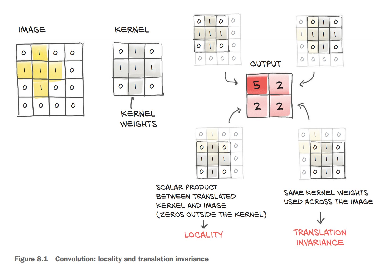
🔹 Mathematical Definition

A convolution takes a small weight matrix (kernel) and slides it over the image.
At each step, it performs an element-wise multiplication between the kernel and the corresponding region of the image, summing the results.

Given a 3×3 filter:

weight = torch.tensor([[w00, w01, w02],
                       [w10, w11, w12],
                       [w20, w21, w22]])

And a single-channel (grayscale) image:

image = torch.tensor([[i00, i01, i02, i03, ..., i0N],
                      [i10, i11, i12, i13, ..., i1N],
                      [i20, i21, i22, i23, ..., i2N],
                      [i30, i31, i32, i33, ..., i3N],
                      ...
                      [iM0, iM1, iM2, iM3, ..., iMN]])

An output pixel is computed as:

o11 = (i11 * w00) + (i12 * w01) + (i13 * w02) +
      (i21 * w10) + (i22 * w11) + (i23 * w12) +
      (i31 * w20) + (i32 * w21) + (i33 * w22)

This process is repeated for every pixel in the image by sliding the filter over it.

How Convolutions Solve Our Problems

🔹 Preserve Local Information → Focus on small regions instead of treating the entire image as a single vector. 🔹 Translation Invariance → Detects patterns anywhere in the image, reducing the need for excessive data augmentation. 🔹 Parameter Efficiency → Instead of learning millions of connections, the model learns a small set of reusable filters.

Convolutions in Action

Convolutional layers in PyTorch provide an efficient way to extract local features from images while maintaining translation invariance.

1. Using nn.Conv2d for Image Data

Handles 2D image data (height × width).
Preserves spatial structure unlike fully connected layers.
Learns local patterns (edges, textures, shapes).

✅ Defining a Convolutional Layer

import torch.nn as nn
conv = nn.Conv2d(in_channels=3, out_channels=16, kernel_size=3)
print(conv)

Conv2d(3, 16, kernel_size=(3, 3), stride=(1, 1))

in_channels=3 → RGB input image.
out_channels=16 → 16 filters for feature extraction.
kernel_size=3 → 3×3 filters scanning the image.

2. Checking Convolution Weights and Biases

Each output channel (feature map) learns a 3×3×3 filter (3 input channels × 3×3 spatial region).

conv.weight.shape, conv.bias.shape

(torch.Size([16, 3, 3, 3]), torch.Size([16]))

(16, 3, 3, 3) → 16 filters, each of size 3×3×3.
(16,) → One bias per output channel.

3. Applying Convolution to an Image

Step 1: Load an image from CIFAR-2 dataset

img, _ = cifar2[0]

Step 2: Add batch dimension (required for nn.Conv2d)

img = img.unsqueeze(0)  # Shape: (1, 3, 32, 32)

Step 3: Pass image through the convolutional layer

output = conv(img)
print(img.shape, output.shape)

(torch.Size([1, 3, 32, 32]), torch.Size([1, 16, 30, 30]))

The output height and width are reduced from 32×32 to 30×30 due to the 3×3 kernel (without padding).

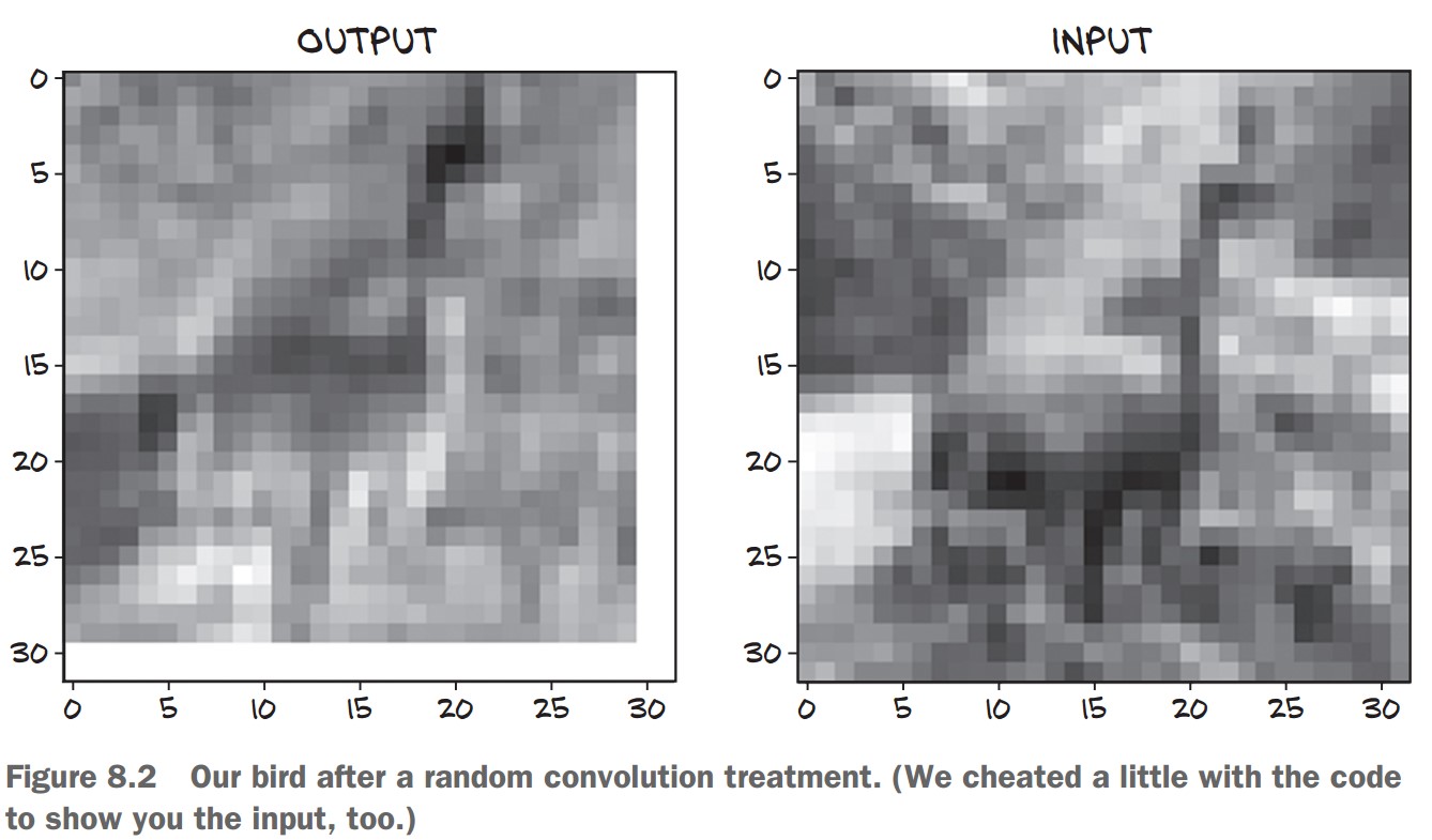
4. Visualizing the Convolution Output

To see how the first filter transforms the image:

import matplotlib.pyplot as plt
plt.imshow(output[0, 0].detach(), cmap='gray')
plt.show()

output[0, 0] → First feature map from the 16 filters.
.detach() → Removes gradient tracking for visualization.
cmap='gray' → Displays in grayscale.

This shows how a single convolution filter highlights patterns in the image! 🎯

Padding in Convolutional Layers

Padding helps preserve the spatial dimensions of an image after applying a convolution operation.

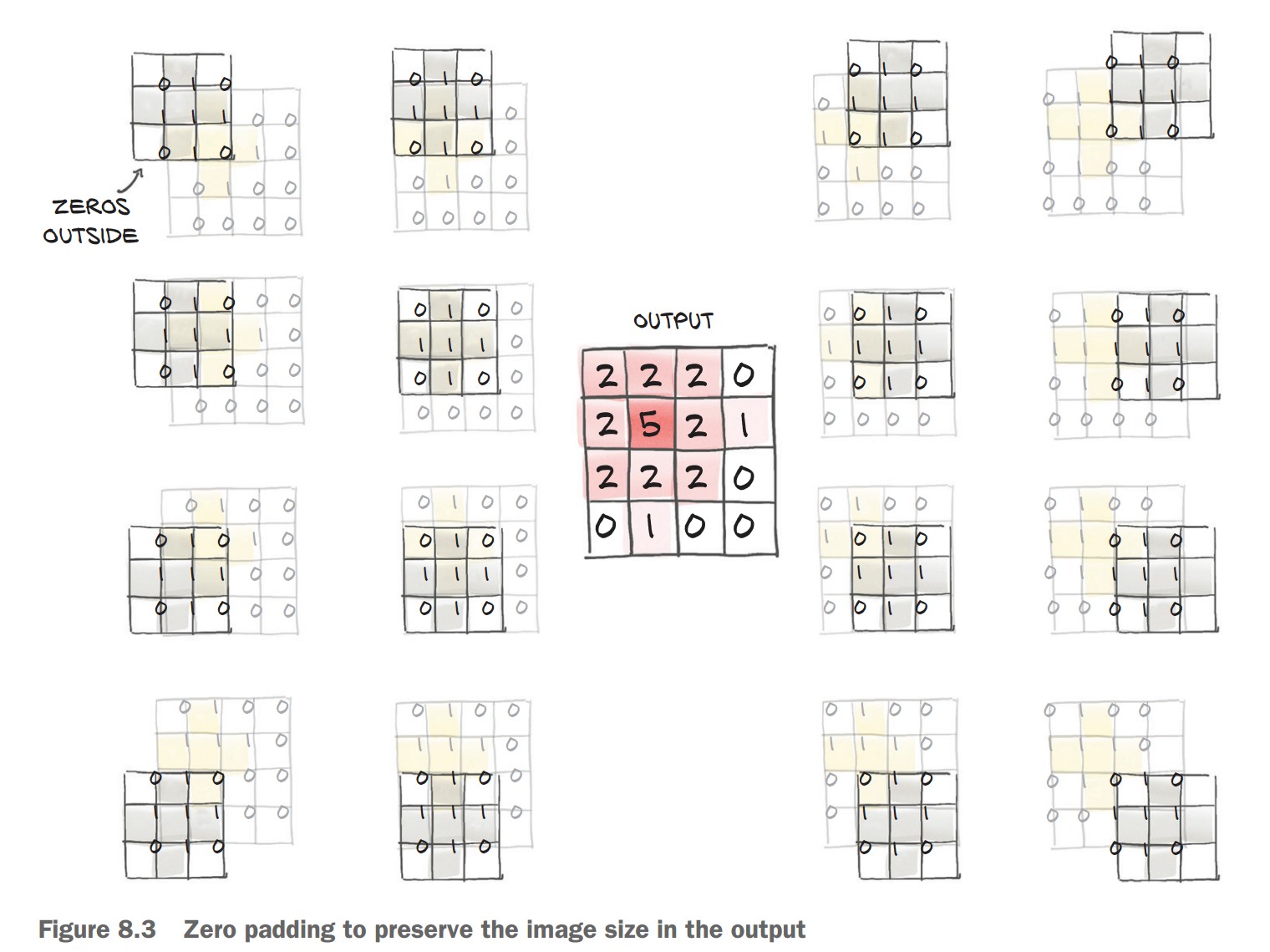
1. Why is Padding Needed?

✅ Convolution Reduces Image Size

A 3×3 filter moves over the image, requiring a 1-pixel border on all sides.
This reduces the output size by 2 pixels per dimension (H_out = H_in - kernel_size + 1).

✅ Padding Adds Ghost Pixels

Padding = 1 adds a 1-pixel border of zeros around the image.
This ensures the output has the same size as the input.

📌 Without Padding (kernel_size=3)

conv = nn.Conv2d(3, 1, kernel_size=3)
output = conv(img.unsqueeze(0))
print(output.shape)

Output: (1, 1, 30, 30) (reduced size)

📌 With Padding (padding=1)

conv = nn.Conv2d(3, 1, kernel_size=3, padding=1)
output = conv(img.unsqueeze(0))
print(output.shape)

Output: (1, 1, 32, 32) (same size as input)

2. Benefits of Padding

✅ Keeps Image Size Unchanged

Ensures output size matches input for easy comparison.

✅ Prevents Information Loss at Borders

Without padding, pixels near edges are underrepresented.

✅ Maintains Compatibility for Advanced Architectures

Needed for skip connections (e.g., U-Nets, ResNets).

3. No Change in Parameters

Padding does not affect the number of trainable parameters in the model.
The weights and biases remain unchanged.

conv.weight.shape, conv.bias.shape

Output:

(torch.Size([1, 3, 3, 3]), torch.Size([1]))

🚀 Padding is essential for deep learning models that need consistent image sizes and improved feature extraction near edges!

Detecting Features with Convolutions

Convolutions allow us to detect patterns such as edges, textures, and shapes in images.

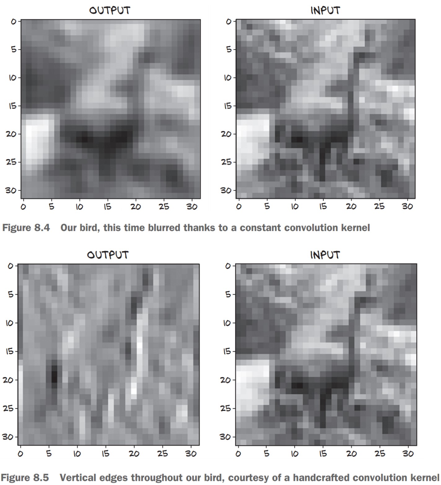
1. Manually Setting Convolution Weights

🔹 Blurring (Smoothing) Filter

Each output pixel is the average of its 3×3 neighbors.
This removes sharp variations and smooths the image.

with torch.no_grad():
    conv.bias.zero_()  # Remove bias
    conv.weight.fill_(1.0 / 9.0)  # Set all weights to 1/9
output = conv(img.unsqueeze(0))
plt.imshow(output[0, 0].detach(), cmap='gray')
plt.show()

🖼 Effect: Produces a blurred version of the image.

2. Edge Detection Using Convolutions

🔹 Vertical Edge Detector Kernel

Highlights vertical edges by computing the difference between left and right pixels.

conv = nn.Conv2d(3, 1, kernel_size=3, padding=1)
with torch.no_grad():
    conv.weight[:] = torch.tensor([
        [-1.0, 0.0, 1.0],
        [-1.0, 0.0, 1.0],
        [-1.0, 0.0, 1.0]
    ])
    conv.bias.zero_()

📌 How It Works:

Computes differences between right and left neighbors.
Detects sharp intensity changes, which indicate edges.

🖼 Effect: Enhances vertical edges in an image.

3. Learning Filters in Deep Learning

🔹 Historically, humans designed filters for different tasks like edge detection and texture analysis. 🔹 With deep learning, CNNs learn the best filters automatically during training.

✅ CNN Layers Learn Different Features

Early layers detect edges and textures.
Deeper layers detect shapes and objects.

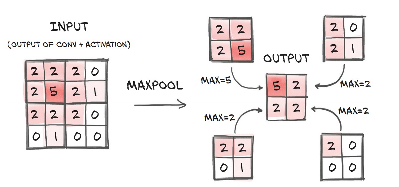
The Need for Pooling (Downsampling)

🔹 Why do we need downsampling?

Small kernels (3×3, 5×5) detect fine details, but we also need to recognize larger patterns.
Instead of using large kernels (which lose locality & increase parameters), we stack multiple convolution layers with downsampling in between.

🔹 How do we downsample?

Average Pooling: Takes the mean of neighboring pixels.
Max Pooling (Most common): Keeps the strongest feature (highest value).
Strided Convolutions: Skips pixels when computing output, keeping more information than pooling.

✅ Max Pooling is widely used since it preserves important features while reducing size.

pool = nn.MaxPool2d(2)  # Pool over 2x2 regions
output = pool(img.unsqueeze(0))
print(img.unsqueeze(0).shape, output.shape)

📌 Effect: Input (32×32) → Output (16×16)

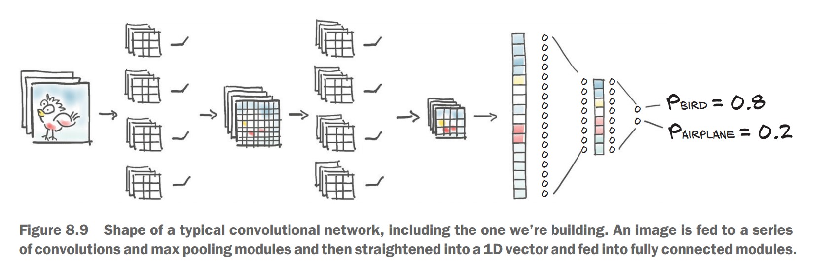
Stacking Convolutions & Pooling

Key Idea: Each layer extracts features at different scales.

First layers detect edges & textures.
Deeper layers detect shapes & objects.

📌 CNN Structure:

First convolution layer increases channels from 3 (RGB) → 16 feature maps.
Then activation (Tanh) and Max Pooling (downsampling).
Another convolution + activation + pooling, reducing spatial size further.

model = nn.Sequential(
    nn.Conv2d(3, 16, kernel_size=3, padding=1),  # 32x32 → 32x32 (16 channels)
    nn.Tanh(),
    nn.MaxPool2d(2),  # 32x32 → 16x16

    nn.Conv2d(16, 8, kernel_size=3, padding=1),  # 16x16 → 16x16 (8 channels)
    nn.Tanh(),
    nn.MaxPool2d(2),  # 16x16 → 8x8
)

✅ This structure helps CNNs recognize larger objects by building features from small patterns.

Transitioning to Fully Connected Layers

🔹 Problem:

CNN layers output 8×8 feature maps, but our classifier needs a 1D vector.
We must flatten the output before feeding it into fully connected (linear) layers.

🔹 Solution: Use view() to reshape output

nn.Linear(8 * 8 * 8, 32),  # 8x8x8 features → 32 neurons
nn.Tanh(),
nn.Linear(32, 2)  # Final layer: 2 outputs (Bird vs. Airplane)

⚠️ Missing Step (Error Fixing): Before passing to nn.Linear, we need to flatten (view() is needed inside forward(), but nn.Sequential lacks explicit visibility).

Subclassing `nn.Module` for Custom Neural Networks

1. Why Subclass nn.Module?

✅ Flexibility: Allows defining custom forward passes beyond just sequential layers. ✅ More Control: Useful for complex architectures, e.g., residual connections (ResNets). ✅ Custom Computation: Needed for non-standard operations (like reshaping before nn.Linear).

2. Creating a Custom CNN Class

We replace nn.Sequential with a subclassed model where we define forward().

📌 Steps:

Initialize layers in __init__.
Define forward pass explicitly.

import torch.nn as nn

class Net(nn.Module):
    def __init__(self):
        super().__init__()
        self.conv1 = nn.Conv2d(3, 16, kernel_size=3, padding=1)
        self.act1 = nn.Tanh()
        self.pool1 = nn.MaxPool2d(2)

        self.conv2 = nn.Conv2d(16, 8, kernel_size=3, padding=1)
        self.act2 = nn.Tanh()
        self.pool2 = nn.MaxPool2d(2)

        self.fc1 = nn.Linear(8 * 8 * 8, 32)  # Flattened output
        self.act3 = nn.Tanh()
        self.fc2 = nn.Linear(32, 2)  # Output (2 classes: Bird/Airplane)

    def forward(self, x):
        out = self.pool1(self.act1(self.conv1(x)))  # Conv → Activation → Pool
        out = self.pool2(self.act2(self.conv2(out)))
        out = out.view(-1, 8 * 8 * 8)  # Flatten before `nn.Linear`
        out = self.act3(self.fc1(out))
        out = self.fc2(out)
        return out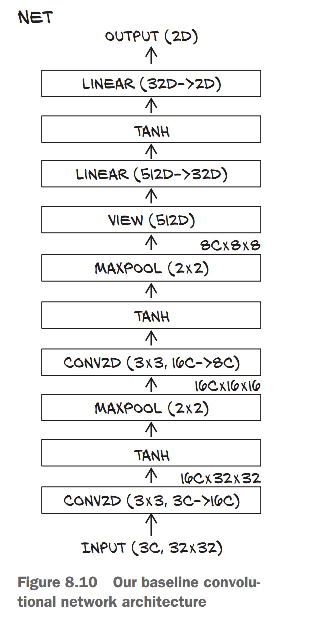

✅ Key Changes from nn.Sequential:

Added view(-1, 8 * 8 * 8) to reshape before Linear.
Layers stored as attributes (self.conv1, etc.) instead of being listed in a container.

3. How PyTorch Tracks Parameters

🔹 Automatically registers layers as submodules when assigned in __init__. 🔹 We can access all parameters using:

model = Net()
num_params = sum(p.numel() for p in model.parameters())
print("Total Parameters:", num_params)

✅ This recursively collects parameters from all submodules (e.g., Conv2d, Linear).

⚠️ Submodules must be top-level attributes!

Avoid storing layers in lists or dictionaries, or PyTorch won’t track them.
If needed, use nn.ModuleList or nn.ModuleDict.

4. Using the Functional API (torch.nn.functional)

✅ Why use it?

No internal state (no parameters).
Simplifies non-trainable layers (e.g., Tanh, MaxPool2d).

🔹 Refactoring forward() with Functional API

import torch.nn.functional as F

class Net(nn.Module):
    def __init__(self):
        super().__init__()
        self.conv1 = nn.Conv2d(3, 16, kernel_size=3, padding=1)
        self.conv2 = nn.Conv2d(16, 8, kernel_size=3, padding=1)
        self.fc1 = nn.Linear(8 * 8 * 8, 32)
        self.fc2 = nn.Linear(32, 2)

    def forward(self, x):
        out = F.max_pool2d(torch.tanh(self.conv1(x)), 2)  # Use functional API
        out = F.max_pool2d(torch.tanh(self.conv2(out)), 2)
        out = out.view(-1, 8 * 8 * 8)
        out = torch.tanh(self.fc1(out))
        out = self.fc2(out)
        return out

✅ Benefits of Functional API:

Removes self.act1 = nn.Tanh() (no need to store state for simple functions).
F.max_pool2d and torch.tanh are stateless, so we call them directly.

5. Running the Model

model = Net()
img, _ = cifar2[0]  # Sample image from dataset
output = model(img.unsqueeze(0))  # Add batch dimension
print(output)

✅ Expected Output: A tensor of shape (1, 2) (logits for Bird/Airplane).

Conclusion

✔ Subclassing nn.Module gives flexibility for custom networks. ✔ PyTorch tracks parameters when assigned in __init__. ✔ Use Functional API (F.tanh, F.max_pool2d) for stateless layers. ✔ Explicit forward() method allows more control over data flow.

Training a Convolutional Neural Network (CNN) in PyTorch

Training Loop for the CNN

📌 Key Steps in Training

Forward pass: Feed images through the model.
Compute loss: Compare predictions to ground truth.
Zero gradients: Clear old gradients before backpropagation.
Backward pass: Compute gradients using loss.backward().
Optimizer step: Update model parameters.

import torch
import torch.nn as nn
import torch.optim as optim
import datetime

def training_loop(n_epochs, optimizer, model, loss_fn, train_loader):
    for epoch in range(1, n_epochs + 1):
        loss_train = 0.0
        for imgs, labels in train_loader:
            outputs = model(imgs)
            loss = loss_fn(outputs, labels)
            optimizer.zero_grad()
            loss.backward()
            optimizer.step()
            loss_train += loss.item()

        if epoch == 1 or epoch % 10 == 0:
            print('{} Epoch {}, Training loss {:.4f}'.format(
                datetime.datetime.now(), epoch, loss_train / len(train_loader)))

✅ Changes from Previous Training Loops:

Now works with convolutional layers (nn.Conv2d) instead of fully connected ones.
Uses cross-entropy loss (nn.CrossEntropyLoss), suitable for classification tasks.

Running Training for 100 Epochs

train_loader = torch.utils.data.DataLoader(cifar2, batch_size=64, shuffle=True)
model = Net()
optimizer = optim.SGD(model.parameters(), lr=1e-2)
loss_fn = nn.CrossEntropyLoss()

training_loop(
    n_epochs=100,
    optimizer=optimizer,
    model=model,
    loss_fn=loss_fn,
    train_loader=train_loader
)

✅ Training Output (Example Results)

Epoch 1, Training loss 0.5634
Epoch 10, Training loss 0.3277
Epoch 20, Training loss 0.3035
Epoch 30, Training loss 0.2825
Epoch 40, Training loss 0.2611
...
Epoch 100, Training loss 0.1614

🔹 Interpretation

Loss decreases steadily, indicating the model is learning.
But loss alone isn't enough—we need accuracy to evaluate performance.

Measuring Accuracy

📌 Steps

Iterate through train & validation sets.
Get model predictions using torch.max().
Compare predictions to ground truth labels.

def validate(model, train_loader, val_loader):
    for name, loader in [("train", train_loader), ("val", val_loader)]:
        correct = 0
        total = 0
        with torch.no_grad():  # Disable gradient calculations
            for imgs, labels in loader:
                outputs = model(imgs)
                _, predicted = torch.max(outputs, dim=1)
                total += labels.shape[0]
                correct += int((predicted == labels).sum())

        print("Accuracy {}: {:.2f}".format(name, correct / total))

train_loader = torch.utils.data.DataLoader(cifar2, batch_size=64, shuffle=False)
val_loader = torch.utils.data.DataLoader(cifar2_val, batch_size=64, shuffle=False)

validate(model, train_loader, val_loader)

✅ Example Accuracy Results

Accuracy train: 0.93
Accuracy val: 0.89

Higher than the 79% accuracy of the fully connected model!
Fewer parameters but better generalization due to convolutions.
Generalization gap: Training accuracy > Validation accuracy (some overfitting).

Saving and Loading the Model

📌 Saving the Model Weights

torch.save(model.state_dict(), "birds_vs_airplanes.pt")

✅ Saves only the model parameters, not the structure.

📌 Loading the Model for Later Use

loaded_model = Net()  # Must define the model architecture
# We will have to make sure we don’t change
# the definition of Net between saving and
# later loading the model state.
loaded_model.load_state_dict(torch.load("birds_vs_airplanes.pt"))

✅ Ensures reusability without retraining.

Training a Convolutional Neural Network (CNN) on a GPU in PyTorch

1. Moving Computation to the GPU

📌 Key Steps

Check if a GPU is available using torch.cuda.is_available().
Move model parameters to the GPU with .to(device).
Move data batches to the GPU before passing them to the model.

import torch

device = torch.device("cuda") if torch.cuda.is_available() else torch.device("cpu")
print(f"Training on device {device}.")

✅ If a GPU is available, PyTorch will use it. Otherwise, it defaults to the CPU.

2. Updating the Training Loop for GPU Support

import datetime

def training_loop(n_epochs, optimizer, model, loss_fn, train_loader):
    for epoch in range(1, n_epochs + 1):
        loss_train = 0.0
        for imgs, labels in train_loader:
            imgs = imgs.to(device)  # Move images to GPU
            labels = labels.to(device)  # Move labels to GPU

            outputs = model(imgs)  # Forward pass
            loss = loss_fn(outputs, labels)

            optimizer.zero_grad()
            loss.backward()  # Backward pass
            optimizer.step()  # Update weights

            loss_train += loss.item()

        if epoch == 1 or epoch % 10 == 0:
            print('{} Epoch {}, Training loss {:.4f}'.format(
                datetime.datetime.now(), epoch, loss_train / len(train_loader)))

✅ Changes for GPU Training:

imgs.to(device) and labels.to(device) move data to the GPU.
Model itself is moved to GPU with model.to(device).

3. Running Training on the GPU

train_loader = torch.utils.data.DataLoader(cifar2, batch_size=64, shuffle=True)

model = Net().to(device)  # Move model to GPU
optimizer = torch.optim.SGD(model.parameters(), lr=1e-2)
loss_fn = nn.CrossEntropyLoss()

training_loop(
    n_epochs=100,
    optimizer=optimizer,
    model=model,
    loss_fn=loss_fn,
    train_loader=train_loader
)

✅ Example Training Output on GPU

Epoch 1, Training loss 0.5718
Epoch 10, Training loss 0.3285
Epoch 20, Training loss 0.2949
Epoch 30, Training loss 0.2696
Epoch 40, Training loss 0.2471
...
Epoch 100, Training loss 0.1567

🔹 Observations

GPU significantly speeds up training (especially for deeper models).
Loss decreases steadily, indicating the model is learning well.

4. Handling GPU-Based Model Checkpoints

📌 Saving the Model Weights

torch.save(model.state_dict(), "birds_vs_airplanes.pt")

✅ GPU Consideration: If saved while on GPU, it will attempt to load back to GPU.

📌 Loading Model Weights Correctly

Ensure compatibility when loading on a different device.
Use map_location=device to move model weights.

loaded_model = Net().to(device)
loaded_model.load_state_dict(torch.load("birds_vs_airplanes.pt", map_location=device))

✅ Prevents errors when moving between CPU and GPU.

Model Design and Regularization in PyTorch

1. Expanding Model Capacity with Width

📌 Key Idea

Increase width (number of channels per convolution layer) to enhance feature extraction.
A wider model has more parameters, increasing learning capacity but also risk of overfitting.

import torch.nn as nn
import torch.nn.functional as F

class NetWidth(nn.Module):
    def __init__(self, n_chans1=32):
        super().__init__()
        self.n_chans1 = n_chans1
        self.conv1 = nn.Conv2d(3, n_chans1, kernel_size=3, padding=1)
        self.conv2 = nn.Conv2d(n_chans1, n_chans1 // 2, kernel_size=3, padding=1)
        self.fc1 = nn.Linear(8 * 8 * n_chans1 // 2, 32)
        self.fc2 = nn.Linear(32, 2)

    def forward(self, x):
        out = F.max_pool2d(torch.tanh(self.conv1(x)), 2)
        out = F.max_pool2d(torch.tanh(self.conv2(out)), 2)
        out = out.view(-1, 8 * 8 * self.n_chans1 // 2)
        out = torch.tanh(self.fc1(out))
        out = self.fc2(out)
        return out

✅ Advantage: Learns richer representations by extracting more diverse features. ⚠️ Risk: More prone to overfitting without proper regularization.

2. Preventing Overfitting with Regularization

📌 L2 Regularization (Weight Decay)

Penalizes large weight values, preventing over-reliance on specific features.
Implemented using weight_decay in the optimizer.

optimizer = torch.optim.SGD(model.parameters(), lr=1e-2, weight_decay=0.001)

✅ More stable training, reduces overfitting.

📌 Dropout Regularization

Randomly sets neuron activations to zero during training, forcing the model to generalize.
Applied after activations to reduce co-adaptation of neurons.

class NetDropout(nn.Module):
    def __init__(self, n_chans1=32):
        super().__init__()
        self.n_chans1 = n_chans1
        self.conv1 = nn.Conv2d(3, n_chans1, kernel_size=3, padding=1)
        self.conv1_dropout = nn.Dropout2d(p=0.4)
        self.conv2 = nn.Conv2d(n_chans1, n_chans1 // 2, kernel_size=3, padding=1)
        self.conv2_dropout = nn.Dropout2d(p=0.4)
        self.fc1 = nn.Linear(8 * 8 * n_chans1 // 2, 32)
        self.fc2 = nn.Linear(32, 2)

    def forward(self, x):
        out = F.max_pool2d(torch.tanh(self.conv1(x)), 2)
        out = self.conv1_dropout(out)
        out = F.max_pool2d(torch.tanh(self.conv2(out)), 2)
        out = self.conv2_dropout(out)
        out = out.view(-1, 8 * 8 * self.n_chans1 // 2)
        out = torch.tanh(self.fc1(out))
        out = self.fc2(out)
        return out

✅ Improves generalization by reducing reliance on individual neurons. ⚠️ Disabled during inference using model.eval().

3. Accelerating Training with Batch Normalization

📌 Key Idea

Normalizes activations per batch to stabilize training and allow higher learning rates.
Reduces dependence on weight initialization.

class NetBatchNorm(nn.Module):
    def __init__(self, n_chans1=32):
        super().__init__()
        self.n_chans1 = n_chans1
        self.conv1 = nn.Conv2d(3, n_chans1, kernel_size=3, padding=1)
        self.conv1_batchnorm = nn.BatchNorm2d(num_features=n_chans1)
        self.conv2 = nn.Conv2d(n_chans1, n_chans1 // 2, kernel_size=3, padding=1)
        self.conv2_batchnorm = nn.BatchNorm2d(num_features=n_chans1 // 2)
        self.fc1 = nn.Linear(8 * 8 * n_chans1 // 2, 32)
        self.fc2 = nn.Linear(32, 2)

    def forward(self, x):
        out = self.conv1_batchnorm(self.conv1(x))
        out = F.max_pool2d(torch.tanh(out), 2)
        out = self.conv2_batchnorm(self.conv2(out))
        out = F.max_pool2d(torch.tanh(out), 2)
        out = out.view(-1, 8 * 8 * self.n_chans1 // 2)
        out = torch.tanh(self.fc1(out))
        out = self.fc2(out)
        return out

✅ Speeds up training and prevents activations from exploding/vanishing. ⚠️ Switches behavior between training and inference using model.train() and model.eval().

Increasing Model Depth for More Complex Representations

The Role of Depth in Neural Networks

📌 Key Idea

Depth enables learning hierarchical features (e.g., edges → textures → objects).
More depth increases model complexity but also makes training harder.
Vanishing gradients issue: deeper layers receive weaker gradient updates.

✅ Solution: Use skip connections (ResNet-style) to improve gradient flow.

Implementing a Deeper Network in PyTorch

📌 Basic Deep CNN Model

Adds an extra convolution layer.
Uses ReLU activation instead of Tanh for better gradient propagation.

import torch.nn as nn
import torch.nn.functional as F

class NetDepth(nn.Module):
    def __init__(self, n_chans1=32):
        super().__init__()
        self.n_chans1 = n_chans1
        self.conv1 = nn.Conv2d(3, n_chans1, kernel_size=3, padding=1)
        self.conv2 = nn.Conv2d(n_chans1, n_chans1 // 2, kernel_size=3, padding=1)
        self.conv3 = nn.Conv2d(n_chans1 // 2, n_chans1 // 2, kernel_size=3, padding=1)
        self.fc1 = nn.Linear(4 * 4 * n_chans1 // 2, 32)
        self.fc2 = nn.Linear(32, 2)

    def forward(self, x):
        out = F.max_pool2d(torch.relu(self.conv1(x)), 2)
        out = F.max_pool2d(torch.relu(self.conv2(out)), 2)
        out = F.max_pool2d(torch.relu(self.conv3(out)), 2)
        out = out.view(-1, 4 * 4 * self.n_chans1 // 2)
        out = torch.relu(self.fc1(out))
        out = self.fc2(out)
        return out

✅ Advantage: Extracts richer features by adding a deeper convolutional layer. ⚠️ Issue: Vanishing gradients can slow down training.

Using Skip Connections (ResNet Style) to Improve Training

📌 Skip Connections (Identity Mapping)

Directly add input of one layer to the output of another.
Helps preserve gradient flow and avoids vanishing gradients.

class NetRes(nn.Module):
    def __init__(self, n_chans1=32):
        super().__init__()
        self.n_chans1 = n_chans1
        self.conv1 = nn.Conv2d(3, n_chans1, kernel_size=3, padding=1)
        self.conv2 = nn.Conv2d(n_chans1, n_chans1 // 2, kernel_size=3, padding=1)
        self.conv3 = nn.Conv2d(n_chans1 // 2, n_chans1 // 2, kernel_size=3, padding=1)
        self.fc1 = nn.Linear(4 * 4 * n_chans1 // 2, 32)
        self.fc2 = nn.Linear(32, 2)

    def forward(self, x):
        out = F.max_pool2d(torch.relu(self.conv1(x)), 2)
        out = F.max_pool2d(torch.relu(self.conv2(out)), 2)
        out1 = out  # Store the intermediate output for skip connection
        out = F.max_pool2d(torch.relu(self.conv3(out)) + out1, 2)  # Skip connection
        out = out.view(-1, 4 * 4 * self.n_chans1 // 2)
        out = torch.relu(self.fc1(out))
        out = self.fc2(out)
        return out

✅ Advantage: Skip connections help retain important gradient information. ⚠️ Issue: Increases memory usage due to additional computations.

Building Very Deep Networks in PyTorch

📌 Standard Approach:

Use modular blocks (e.g., Conv + BatchNorm + ReLU).
Dynamically stack layers in a loop.

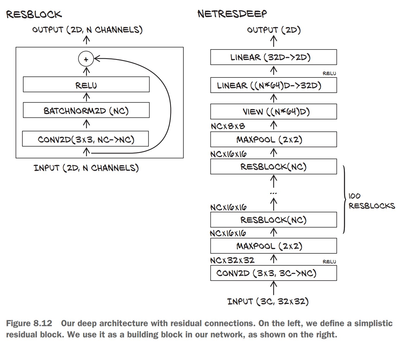
📌 Creating a Residual Block (ResBlock)

Adds batch normalization to stabilize gradients.
Uses Kaiming initialization for better convergence.

class ResBlock(nn.Module):
    def __init__(self, n_chans):
        super(ResBlock, self).__init__()
        self.conv = nn.Conv2d(n_chans, n_chans, kernel_size=3, padding=1, bias=False)
        self.batch_norm = nn.BatchNorm2d(num_features=n_chans)
        torch.nn.init.kaiming_normal_(self.conv.weight, nonlinearity='relu')
        torch.nn.init.constant_(self.batch_norm.weight, 0.5)
        torch.nn.init.zeros_(self.batch_norm.bias)

    def forward(self, x):
        out = self.conv(x)
        out = self.batch_norm(out)
        out = torch.relu(out)
        return out + x  # Skip connection

✅ Advantage: Helps build deeper models while maintaining stable training.

📌 Creating a Deep Residual Network

Stacks multiple ResBlocks dynamically.

class NetResDeep(nn.Module):
    def __init__(self, n_chans1=32, n_blocks=10):
        super().__init__()
        self.n_chans1 = n_chans1
        self.conv1 = nn.Conv2d(3, n_chans1, kernel_size=3, padding=1)
        self.resblocks = nn.Sequential(*(n_blocks * [ResBlock(n_chans=n_chans1)]))
        self.fc1 = nn.Linear(8 * 8 * n_chans1, 32)
        self.fc2 = nn.Linear(32, 2)

    def forward(self, x):
        out = F.max_pool2d(torch.relu(self.conv1(x)), 2)
        out = self.resblocks(out)  # Pass through multiple ResBlocks
        out = F.max_pool2d(out, 2)
        out = out.view(-1, 8 * 8 * self.n_chans1)
        out = torch.relu(self.fc1(out))
        out = self.fc2(out)
        return out

✅ Advantage: Scales to 100+ layers without gradient vanishing issues. ⚠️ Issue: Requires careful hyperparameter tuning for stability.

Weight Initialization for Deep Networks

📌 Why Initialization Matters

Poor initialization can lead to slow convergence or unstable gradients.
Kaiming (He) Initialization works best for ReLU-based networks.

torch.nn.init.kaiming_normal_(layer.weight, nonlinearity='relu')

✅ Ensures stable gradients throughout the network.

Key Takeaways on Model Evolution and Future Challenges

The Ever-Changing Nature of Neural Networks

📌 Deep Learning Evolves Rapidly

New architectures emerge frequently, making older models outdated.
Understanding core concepts helps adapt to new techniques.
The ability to translate research papers into PyTorch code is essential.

✅ Takeaway: Focus on learning principles rather than just memorizing specific architectures.

Our Image Classifier: Achievements & Limitations

📌 What We Accomplished

✔ Built a convolutional neural network (CNN) to classify birds vs. airplanes.
✔ Explored model depth, width, regularization, and training techniques.
✔ Improved accuracy while reducing overfitting.

📌 Remaining Challenges

🔴 Object Localization: Our model works for cropped images but can't find birds/airplanes in larger scenes.
🔴 Overgeneralization: Model confidently misclassifies unseen objects (e.g., a cat as a bird).
🔴 Real-World Robustness: Uncertain performance on noisy or unexpected inputs.

ch8.convolution_to_generalize

Ch 8. Using convolutions to generalize

The Case for Convolutions in Neural Networks

What is a Convolution?

How Convolutions Solve Our Problems

Convolutions in Action

Padding in Convolutional Layers

Detecting Features with Convolutions

3. Learning Filters in Deep Learning

The Need for Pooling (Downsampling)

Transitioning to Fully Connected Layers

Subclassing nn.Module for Custom Neural Networks

Training a Convolutional Neural Network (CNN) in PyTorch

Training a Convolutional Neural Network (CNN) on a GPU in PyTorch

Model Design and Regularization in PyTorch

Increasing Model Depth for More Complex Representations

Using Skip Connections (ResNet Style) to Improve Training

📌 Creating a Residual Block (ResBlock)

📌 Creating a Deep Residual Network

Weight Initialization for Deep Networks

Key Takeaways on Model Evolution and Future Challenges

Subclassing `nn.Module` for Custom Neural Networks