ch7.processing_data
Ch 7. Processing data
Introduction
What foundational issues should workflows address when handling data?
Workflows must solve how to consume and produce data efficiently and reliably. This includes:
1. What types of data sources might a workflow interact with?
- Prototyping: local files (e.g., CSVs via
IncludeFile) - Small/medium companies: relational databases (e.g., PostgreSQL)
- Larger systems:
- Federated query engines: Trino (Presto)
- Data lakes: cloud-based storage with tools like:
- Apache Flink (streaming)
- Apache Iceberg (metadata handling)
- Apache Spark (batch processing)
2. What data types and modalities should be considered?
- Structured data: tables, columns, SQL queries
- Unstructured data: free text, images, audio
- Semi-structured data: JSON, logs, event streams (partially structured)
3. What are the core concerns for data access?
-
Performance:
- Fast, efficient loading of large datasets
- Avoid bottlenecks that slow down prototyping
-
Data Selection:
- Find relevant subsets efficiently (typically via SQL)
- Support for structured and semi-structured data
-
Feature Engineering:
- Transform raw data into model-friendly formats
- Preprocessing, encoding, aggregations, etc.
4. How often should the application react to new data?
-
Batch processing:
- Triggered at intervals (e.g., every 15 minutes)
- Simpler, easier to manage
-
Streaming:
- Real-time, continuous updates
- More complex infrastructure
5. Who owns the data access logic?
- Varies by organization, but typical roles include:
- Data engineers: ensure raw data is available and clean
- Data scientists: explore and model the data
Why does this matter?
Efficient data access and transformation patterns directly impact:
- Speed of iteration (prototyping loop)
- Workflow reliability and scalability
- Collaboration between engineering and data science teams
Although loading data from a data warehouse to a workflow seems like a technical detail, it impacts how teams work, how infrastructure is architected, and how scalable and efficient workflows become.
What is the traditional approach to data access in analytics?
- Data stays inside the warehouse.
- Applications express their needs via complex SQL queries.
- The warehouse returns a small, filtered result to tools like Tableau dashboards.
- Benefits:
- Centralized control over data.
- Efficient for business intelligence queries.
- Limitations for ML:
- Cannot run compute-heavy tasks like model training.
- Tightly couples compute with the data layer, limiting scalability.
Why doesn’t this work well for machine learning?
- ML applications often need simple but high-volume queries like
SELECT * FROM table. - ML workloads require:
- Bulk data access
- Decoupling of compute from data
- Autoscaling compute resources, such as GPU-backed instances
- Problems encountered:
- Data warehouses may be inefficient at handling large reads.
- Client libraries often aren’t optimized for bulk transfer.
What is the case for decoupling data and compute?
- Enables use of optimal compute layers (e.g., AWS Batch, GPUs).
- Allows data scientists to iterate freely, without affecting production databases.
- Reduces coordination overhead between teams.
- Tradeoff: Loses centralized control over how data is used, increasing the need for proper data access management.
How do ML and BI applications differ in data access?
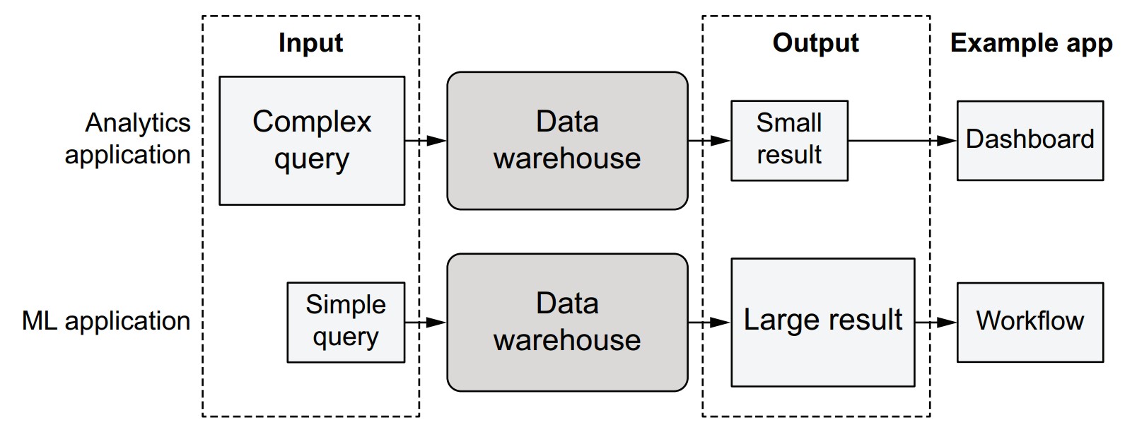
| Characteristic | BI (e.g., Tableau) | ML Workflows |
|---|---|---|
| Query complexity | High | Low (SELECT *) |
| Result size | Small | Large (full table) |
| Optimized for | Filtered insights | Bulk ingestion |
| Performance bottleneck | Query logic | Data transfer/loading |
| Compute needs | Light (local/client-side) | Heavy (external, autoscaled compute) |
S3
How does loading data from S3 compare to local files?
- Preferred by data scientists: Local files are simple, fast, stable, and universally supported.
- Downsides of local files:
- Not suitable for cloud workflows.
- Require manual updates.
- Don’t adhere to governance policies.
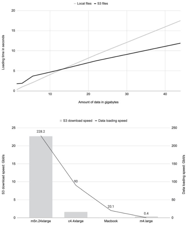
Why use S3 instead?
-
Pros:
- Cloud-compatible and governance-friendly.
- Supports scalable workflows.
- Can outperform local files, especially for large datasets.
-
Benchmark Summary (based on listing
s3benchmark.py):- When dataset fits in memory, S3 loading uses disk cache, enabling very high read speeds.
- Throughput depends on:
- Instance size: Larger instances (e.g.,
m5n.24xlarge) = higher performance. - File size: Avoid many small files; prefer tens of MB or larger.
- Region alignment: Run compute in same region as the S3 bucket to avoid latency and transfer costs.
- Instance size: Larger instances (e.g.,
Key code concepts from the S3 benchmark
-
Listing S3 files:
files = list(s3.list_recursive([URL]))[:num] -
Downloading multiple objects:
loaded = s3.get_many([f.url for f in files]) -
Parallel file reading:
parallel_map(lambda x: len(open(x, 'rb').read()), files) -
Disk cache advantage:
- S3-loaded files stay in memory (via OS-level disk cache) if dataset fits.
- Local files are often read from disk, making them slower on under-provisioned machines.
Best practices for loading from S3
- Use
@resourcesto allocate enough memory for datasets to stay in RAM. - Use large files (tens of MB or more) for optimal S3 throughput.
- Favor cloud-based instances for benchmarking or heavy workloads.
- Prefer
metaflow.S3over ad hoc S3 clients for consistency and performance. - Keep compute and S3 storage in the same AWS region.
s3benchmark.py
This script benchmarks the performance of loading data from either:
- Local files (
--local_dirspecified), or - S3 (via
metaflow.S3) if no local directory is given.
import os
from metaflow import FlowSpec, step, Parameter, S3, profile, parallel_map

URL = "s3://commoncrawl/crawl-data/CC-MAIN-2021-25/segments/1623488519735.70/wet/"


def load_s3(s3, num):
    files = list(s3.list_recursive([URL]))[:num]
    total_size = sum(f.size for f in files) / 1024**3  # in GB
    stats = {}

    with profile("downloading", stats_dict=stats):
        loaded = s3.get_many([f.url for f in files])

    s3_gbps = (total_size * 8) / (stats["downloading"] / 1000.0)
    print("S3->EC2 throughput: %2.1f Gb/s" % s3_gbps)
    return [obj.path for obj in loaded]


class S3BenchmarkFlow(FlowSpec):

    local_dir = Parameter("local_dir", help="Read local files from this directory")

    num = Parameter("num_files", help="Maximum number of files to read", default=50)

    @step
    def start(self):
        with S3() as s3:
            with profile("Loading and processing"):
                if self.local_dir:
                    files = [
                        os.path.join(self.local_dir, f)
                        for f in os.listdir(self.local_dir)
                    ][: self.num]
                else:
                    files = load_s3(s3, self.num)

                print("Reading %d objects" % len(files))

                stats = {}
                with profile("reading", stats_dict=stats):
                    size = (
                        sum(parallel_map(lambda x:
                          len(open(x, "rb").read()), files)) / 1024**3
                    )  # in GB

                read_gbps = (size * 8) / (stats["reading"] / 1000.0)
                print("Read %2.1f GB. Throughput: %2.1f Gb/s" % (size, read_gbps))

        self.next(self.end)

    @step
    def end(self):
        pass


if __name__ == "__main__":
    S3BenchmarkFlow()
profile: Measures timing for download and read phases.parallel_map: Leverages multiple CPU cores to load data in parallel.S3()context: Automatically handles cleanup of temporary files.--local_dir: Optional CLI parameter to test local file performance.@resources: Add this if running large workloads on Batch for better performance.
-
Run locally:
python s3benchmark.py run --num_files 10 -
Run with cloud compute:
python s3benchmark.py run --with batch:memory=16000 -
Run with local files:
python s3benchmark.py run --num_files 10 --local_dir local_data
Recommendations
- Use S3 for all scalable workflows.
- Benchmark file loading realistically using appropriate instances.
- Choose instance size based on dataset size to ensure memory fits.
Working with tabular data
- Shifts focus from raw byte movement to structured/semi-structured tabular data, typically handled as dataframes.
- Structured data is common in business data science, such as data from relational databases.
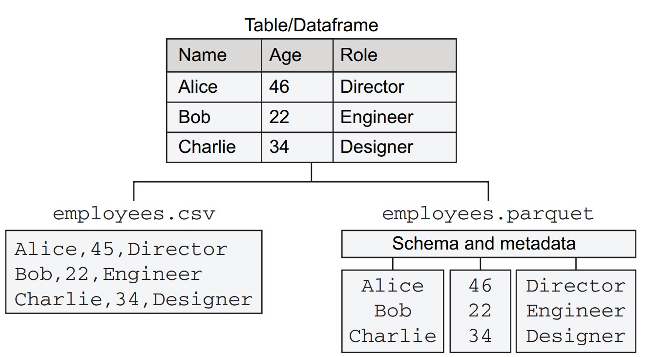
- A tabular dataset with three columns:
name,age,role, and three rows for employee records.- CSV (Comma-Separated Values): Plain text, one row per line, values separated by commas.
- Parquet: A column-oriented binary format.
How do Parquet and CSV compare for structured data?
-
Column Storage:
- Parquet stores each column independently.
- Benefits include type-specific compression and efficient column-based querying.
-
Schema Handling:
- Parquet includes an explicit schema and metadata.
- CSV treats all values as strings, lacking schema awareness.
-
Efficiency:
- Columnar layout in Parquet supports efficient access, e.g.,
SELECT name, role FROM tableorSELECT AVG(age). - Parquet uses binary compression, reducing file size and transfer time.
- Columnar layout in Parquet supports efficient access, e.g.,
How is Parquet read into memory and what library is used?
- CSV: Read using Python’s built-in
csvmodule. - Parquet: Read using Apache Arrow, which:
- Decodes Parquet.
- Offers efficient in-memory representation for processing.
How does the benchmark flow (ParquetBenchmarkFlow) operate?
import os
from metaflow import FlowSpec, step, conda_base, resources, S3, profile

URL = 's3://ursa-labs-taxi-data/2014/12/data.parquet'

@conda_base(python='3.8.10',
        libraries={'pyarrow': '5.0.0', 'pandas': '1.3.2', 'memory_profiler': '0.58.0'})
class ParquetBenchmarkFlow(FlowSpec):

    @step
    def start(self):
        import pyarrow.parquet as pq
        with S3() as s3:
            res = s3.get(URL)
            table = pq.read_table(res.path)
            os.rename(res.path, 'taxi.parquet')
        table.to_pandas().to_csv('taxi.csv')
        self.stats = {}
        self.next(self.load_csv, self.load_parquet, self.load_pandas)

    @step
    def load_csv(self):
        with profile('load_csv', stats_dict=self.stats):
            import csv
            with open('taxi.csv') as csvfile:
                for row in csv.reader(csvfile):
                    pass
        self.next(self.join)

    @step
    def load_parquet(self):
        with profile('load_parquet', stats_dict=self.stats):
            import pyarrow.parquet as pq
            table = pq.read_table('taxi.parquet')
        self.next(self.join)

    @step
    def load_pandas(self):
        with profile('load_pandas', stats_dict=self.stats):
            import pandas as pd
            df = pd.read_parquet('taxi.parquet')
        self.next(self.join)

    @step
    def join(self, inputs):
        for inp in inputs:
            print(list(inp.stats.items())[0])
        self.next(self.end)

    @step
    def end(self):
        pass

if __name__ == '__main__':
ParquetBenchmarkFlow()-
start:
- Downloads Parquet from S3.
- Reads it with PyArrow.
- Converts to CSV using pandas for benchmarking.
-
load_csv:
- Reads all rows from CSV with
csv.reader.
- Reads all rows from CSV with
-
load_parquet:
- Loads data using PyArrow (
read_table).
- Loads data using PyArrow (
-
load_pandas:
- Loads Parquet using pandas (
read_parquet).
- Loads Parquet using pandas (
-
join:
- Prints load timing from each method.
-
Run with:
python parquet_benchmark.py --environment=conda run --max-workers 1 -
Use
--max-workers 1to ensure sequential execution for fair timing. -
startstep takes longer (downloads 319MB file, converts to 1.6GB CSV). -
Use
resumeto skip slowstartduring iteration (e.g.,resume load_csv).
What are the performance results?
- load_parquet: Fastest (~973 ms).
- load_pandas: Slower (~1853 ms).
- load_csv: Slowest (~19.5 s). If data retained in memory, time jumps to ~70s and ~20GB RAM usage.
What is the takeaway regarding file format choice?
- Recommendation: Use Parquet whenever feasible.
- Exceptions:
- Sharing small datasets.
- Environments that can't handle Parquet.
- Simpler inspection with CSV using standard tools (though Parquet viewers exist).
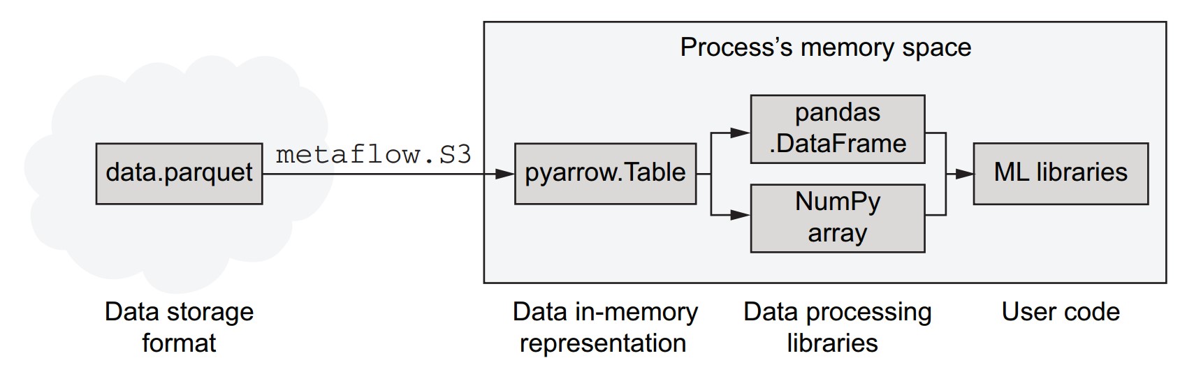
The in-memory data stack
What are the core components and relationships in the in-memory data stack?
- Parquet is a data storage format that is more efficient than CSV for storing and transferring data.
- Parquet files can be loaded efficiently from cloud storage like S3 using libraries such as
metaflow.S3. - Arrow (specifically PyArrow in Python) decodes Parquet files into an efficient in-memory representation.
- Arrow's in-memory data structures can be used directly or passed to other libraries like pandas and NumPy.
- Arrow's superpower: avoids unnecessary data copying, enabling high-performance processing in memory-constrained or speed-critical workflows.
- pandas is user-friendly and rich in data manipulation features but can be memory-intensive and slower compared to Arrow.
- Depending on the task:
- Use pandas for data wrangling tasks.
- Use Arrow or NumPy when memory and performance are priorities.
- Prefer direct consumption by ML libraries that accept Arrow or NumPy formats.
How can we profile memory usage in Metaflow steps?
- Use the
memory_profilerlibrary to monitor memory consumption. - A decorator
@profile_memoryis defined to wrap Metaflow steps and record peak memory usage.
from functools import wraps

def profile_memory(mf_step):
    @wraps(mf_step)
    def func(self):
        from memory_profiler import memory_usage
        self.mem_usage = memory_usage(
            (mf_step, (self,), {}),
            max_iterations=1,
            max_usage=True,
            interval=0.2
        )
return func- Save this in a file named
metaflow_memory.py. - To use:
- Import it:
from metaflow_memory import profile_memory - Ensure
memory_profileris listed in@conda_base:@conda_base(libraries={'memory_profiler': '0.58.0'}) - Apply to steps like:
@profile_memory
@step
def load_csv(self):
    ...
- Import it:
How can memory usage be collected and displayed across branches?
- Add the decorator to every branch where profiling is needed.
- In the
joinstep, access and print each branch’s memory usage:
@step
def join(self, inputs):
    for inp in inputs:
        print(list(inp.stats.items())[0], inp.mem_usage)
self.next(self.end)- To simulate peak memory usage when reading CSV:
- Use
list(csv.reader(csvfile))instead of looping through and discarding rows. - This may require >16 GB RAM.
- Use
What were the results of the CSV vs. Arrow vs. pandas memory benchmark?
- Holding CSV data in memory as raw Python objects:
- Consumed nearly 17 GB RAM.
- Using pandas:
- About 1 GB more memory than Arrow, due to additional Python-friendly structures.
- Using Arrow:
- Most memory-efficient, ideal for large datasets.
What is the memory-efficiency recommendation?
- Avoid storing rows as Python objects when possible.
- Converting to pandas should be avoided if memory is a concern.
- Prefer Arrow or NumPy for memory- and performance-sensitive applications.
What to do when dataset size exceeds memory limits?
- When data exceeds available instance memory (e.g., beyond
@resources(memory=256000)):- Use upstream infrastructure like query engines to filter, join, and prepare data before processing.
- This allows workflows to handle arbitrary volumes of raw data in manageable chunks.
Interfacing with data infrastructure
Why should data science workflows integrate with existing data infrastructure?
- Most companies already have centralized data infrastructure to support analytics, product features, and other applications.
- Consistency in data use across applications—including data science—is important.
- Differences in usage:
- Data science workflows often require large-scale data extracts (tens to hundreds of GB).
- Compute demands are higher for model training compared to dashboards or analytics apps.
- Despite differences, it's beneficial to align data science and data infrastructure to avoid duplication and reduce operational overhead.
What are the layers of modern data infrastructure?
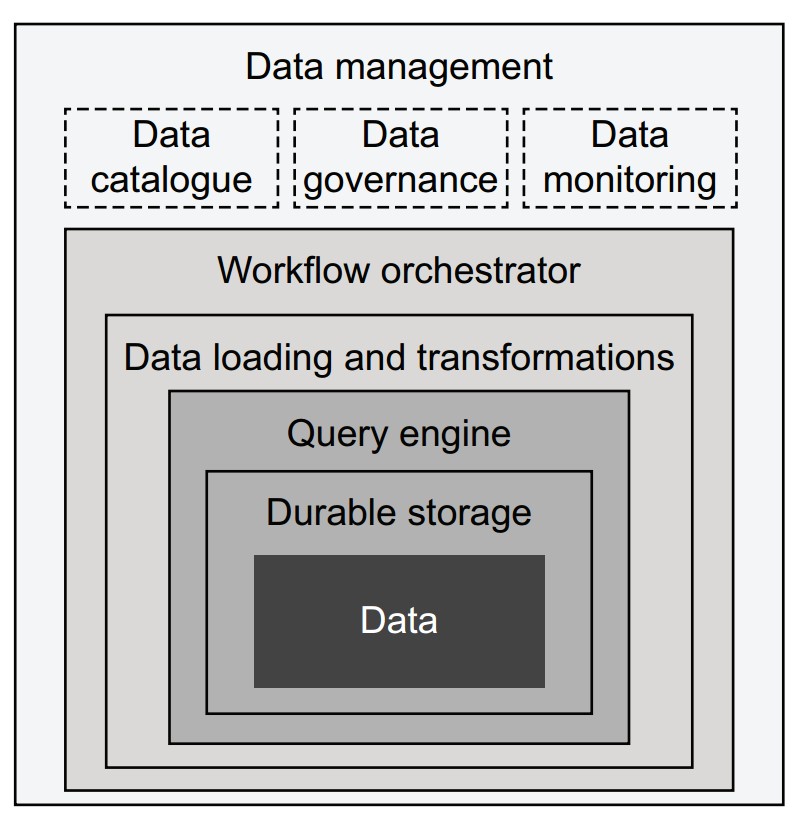
Each component adds capability, starting from the core (data) outward:
- Data: Stored as files (CSV, Parquet) or in databases; assumed to be already available.
- Durable storage:
- E.g., AWS S3, replicated databases.
- Can be enhanced with metadata layers (e.g., Apache Hive, Iceberg) to support query engines.
- Query engine:
- Translates queries (e.g., SQL) into data subsets.
- Traditional: tightly integrated stacks (Postgres, Teradata).
- Modern: loosely coupled (Trino/Presto, Apache Spark); streaming options include Apache Druid, Pinot.
- ETL / ELT systems:
- Move and transform data between systems.
- ELT model (e.g., Snowflake, Spark) loads raw data first, then transforms.
- Tools: DBT (transform management), Great Expectations (data quality).
- Workflow orchestrator:
- Executes DAG-based pipelines (ETL or data science).
- Examples: AWS Step Functions, Apache Airflow, Apache Flink (streaming).
- Data management:
- Tools like Amundsen for cataloging.
- Governance, monitoring, and policy enforcement (e.g., access control, lineage tracking).
How does the data science infrastructure integrate with data infrastructure?
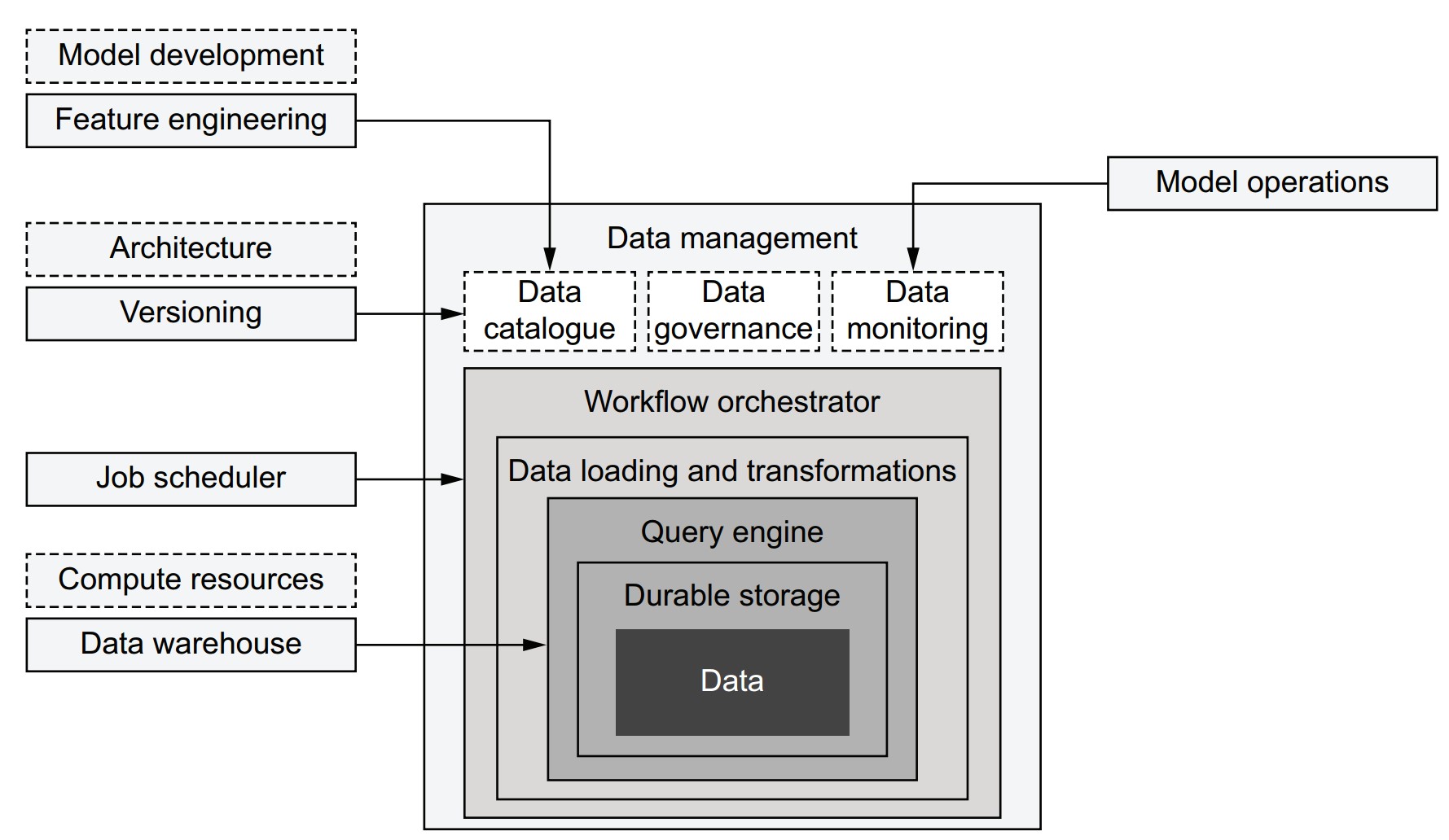
- Integration increases over time as systems evolve.
- Components often shared:
- Job scheduling: Centralized orchestrators can manage both data and data science workflows (e.g., triggering model retraining after data updates).
- Data versioning: Data catalogs can support lineage from raw data to models (e.g., tracking with Metaflow artifacts).
- Monitoring: Source data monitoring can prevent model failure.
- Feature engineering: Catalogs help discover usable features; some double as feature stores.
- Python libraries often act as connectors (e.g., AWS Data Wrangler).
- Components should be adopted incrementally, based on evolving needs.
How can work be divided between data engineers and data scientists?
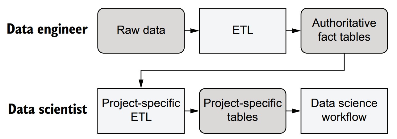
-
Data Engineer responsibilities:
- Acquire and curate raw data.
- Ensure data quality, validity, and structure.
- Produce stable, authoritative datasets (e.g., structured tables).
- Should avoid making interpretive transformations; focus on raw facts.
-
Data Scientist responsibilities:
- Build, deploy, and maintain data science workflows and models.
- Create project-specific tables/views based on curated datasets.
- Can iterate quickly and adjust feature engineering independently.
- Responsible for performance-sensitive aspects like partitioning and layout.
Why is modern infrastructure critical to enable this division?
- Query engines must be robust enough to tolerate less optimized queries from non-experts.
- In the past, data warehouses could be easily overloaded by inefficient queries.
- Modern systems isolate and handle workloads gracefully, allowing safe use by both engineers and scientists.
Preparing datasets in SQL
- Use SQL engines (e.g., Trino, Spark) or warehouses (e.g., Redshift, Snowflake) to prepare datasets for data science workflows.
- Demonstrate dataset preparation using AWS Athena, a managed query engine compatible with the Apache Hive metastore.
- Use CTAS (Create Table As Select) queries to create optimized subsets of data for efficient consumption.
- Employ AWS Data Wrangler to interface with Athena and simplify reading/writing from AWS services.
Dataset preparation
-
Upload source data to S3 and register it as a table with schema metadata.
-
Athena metadata format is compatible with Apache Hive.
-
Partitioning strategy is used to improve query performance by organizing data into subdirectories by month.
Example S3 path structure:
s3://my-metaflow-bucket/metaflow/data/TaxiDataLoader/12/nyc_taxi/month=11/file.parquet- Only the suffix
month=11is crucial for partitioning. - Prefix paths will differ depending on Metaflow configuration.
- Only the suffix
- Ensure IAM user or Batch role has
AmazonAthenaFullAccesspolicy. - Set AWS region via
AWS_DEFAULT_REGION(e.g.,us-east-1).
- Load a year’s worth of data (~160 million rows).
- Partition the table by month using directory structure for optimized querying.
- Convert schema from Parquet to Hive-compatible format.
How does the Metaflow TaxiDataLoader workflow implement this logic?
from metaflow import FlowSpec, Parameter, step, conda, profile, S3

GLUE_DB = 'dsinfra_test'
URL = 's3://ursa-labs-taxi-data/2014/'

TYPES = {'timestamp[us]': 'bigint', 'int8': 'tinyint'}

class TaxiDataLoader(FlowSpec):

    table = Parameter('table', help='Table name', default='nyc_taxi')

    @conda(python='3.8.10', libraries={'pyarrow': '5.0.0'})
    @step
    def start(self):
        import pyarrow.parquet as pq

        def make_key(obj):
            key = '%s/month=%s/%s' % tuple([self.table] + obj.key.split('/'))
            return key, obj.path

        def hive_field(f):
            return f.name, TYPES.get(str(f.type), str(f.type))

        with S3() as s3down:
            with profile('Dowloading data'):
                loaded = list(map(make_key, s3down.get_recursive([URL])))
            table = pq.read_table(loaded[0][1])
            self.schema = dict(map(hive_field, table.schema))

            with S3(run=self) as s3up:
                with profile('Uploading data'):
                    uploaded = s3up.put_files(loaded)
                key, url = uploaded[0]
                self.s3_prefix = url[:-(len(key) - len(self.table))]
        self.next(self.end)

    @conda(python='3.8.10', libraries={'awswrangler': '1.10.1'})
    @step
    def end(self):
        import awswrangler as wr
        try:
            wr.catalog.create_database(name=GLUE_DB)
        except:
            pass
        wr.athena.create_athena_bucket()
        with profile('Creating table'):
            wr.catalog.create_parquet_table(
                database=GLUE_DB,
                table=self.table,
                path=self.s3_prefix,
                columns_types=self.schema,
                partitions_types={'month': 'int'},
                mode='overwrite'
            )
            wr.athena.repair_table(self.table, database=GLUE_DB)

if __name__ == '__main__':
TaxiDataLoader()-
startstep:- Copies and reorganizes Parquet files to use partitioning structure.
- Extracts and transforms schema from Parquet to Hive-compatible format.
-
endstep:- Creates a Glue database (
dsinfra_test) if it doesn’t exist. - Sets up Athena result bucket.
- Registers the table using
awswrangler.catalog.create_parquet_table. - Calls
repair_tableto register partitions.
- Creates a Glue database (
python taxi_loader.py --environment=conda run- Prefer running on AWS Batch or a cloud workstation due to ~4.2GB data volume.
- Verify in Athena console:
- Table
nyc_taxishould appear underdsinfra_test. - Run test query:
SELECT * FROM nyc_taxi LIMIT 10;
- Table
How can project-specific CTAS queries be integrated into a workflow?
- Avoid decoupling SQL logic from data science workflows by executing queries inside flows.
- Use a CTAS (Create Table As Select) approach within the flow to generate result tables dynamically.
- Store SQL in external
.sqlfiles for better IDE support and maintainability.
What does the sample SQL file (sql/taxi_etl.sql) look like?
SELECT * FROM nyc_taxi
WHERE hour(from_unixtime(pickup_at / 1000)) BETWEEN 9 AND 17- Converts
pickup_atfrom milliseconds to seconds. - Filters for business-hour rides (9 a.m. to 5 p.m.).
How is the CTAS query executed in the flow?
from metaflow import FlowSpec, project, profile, S3, step, current, conda

GLUE_DB = 'dsinfra_test'

@project(name='nyc_taxi')
class TaxiETLFlow(FlowSpec):

    def athena_ctas(self, sql):
        import awswrangler as wr
        table = 'mf_ctas_%s' % current.pathspec.replace('/', '_')
        self.ctas = "CREATE TABLE %s AS %s" % (table, sql)
        with profile('Running query'):
            query = wr.athena.start_query_execution(self.ctas, database=GLUE_DB)
            output = wr.athena.wait_query(query)
            loc = output['ResultConfiguration']['OutputLocation']
            with S3() as s3:
                return [obj.url for obj in s3.list_recursive([loc + '/'])]

    @conda(python='3.8.10', libraries={'awswrangler': '1.10.1'})
    @step
    def start(self):
        with open('sql/taxi_etl.sql') as f:
            self.paths = self.athena_ctas(f.read())
        self.next(self.end)

    @step
    def end(self):
        pass

if __name__ == '__main__':
TaxiETLFlow()-
athena_ctasmethod:- Converts the SQL string into a CTAS query.
- Runs it using AWS Wrangler.
- Waits for query completion and stores output file paths in
self.paths.
-
startstep:- Reads SQL file content.
- Runs the CTAS process and stores results.
-
Artifacts stored:
self.ctas: the executed SQL statement.self.paths: list of output file locations.
How do you run the flow and ensure .sql file inclusion?
python taxi_etl.py --environment=conda --package-suffixes .sql run--package-suffixes .sqlensures SQL files are bundled with the flow.
How does this pattern support traceability and debugging?
- CTAS table names include the run and task IDs, e.g.,
mf_ctas_TaxiETLFlow_1631494834745839_start_1. - By logging:
- The SQL query (
self.ctas) - The result locations (
self.paths)
- The SQL query (
- Enables full data lineage: from raw data → queries → results → models.
How does versioned storage work with S3(run=self)?
- Automatically stores data in run-specific paths.
- Enables:
- Isolation across runs.
- Versioning without collisions.
- Facilitates reproducibility and traceability of data across runs.
What are best practices for managing old CTAS query results?
-
S3 Lifecycle Policy:
- Configure automatic deletion of objects at result paths (e.g., after 30 days).
-
Glue Table Cleanup:
- Delete table metadata manually or via:
aws glue batch-delete-table - Or programmatically using AWS Data Wrangler:
wr.catalog.delete_table(database="dsinfra_test", table="table_name")
- Delete table metadata manually or via:
Miscellaneous Notes
- You can replicate the CTAS pattern with Spark, Redshift, or Snowflake.
- Suitable for integrating scalable query processing into data science workflows.
- Compatible with production schedulers for routine ETL tasks.
Distributed data processing
- Single-instance loading (e.g., via Parquet + Arrow + NumPy) is fast and efficient when data fits in memory.
- Limits arise when:
- Dataset size exceeds memory.
- Processing becomes too slow on one machine.
- In such cases, distribute computation across multiple instances using Metaflow’s
foreach.
What are common distributed data processing use cases?
- Subset-specific processing (e.g., per country, per hour).
- Efficient data preprocessing:
- Extract with SQL (e.g., via CTAS).
- Preprocess further in Python.
- Sharded data processing:
- Input split into chunks.
- Processed in parallel.
- Results aggregated in a
joinstep (MapReduce style).
How does the helper function for visualization work?
from io import BytesIO

CANVAS = {
    'plot_width': 1000,
    'plot_height': 1000,
    'x_range': (-74.03, -73.92),
    'y_range': (40.70, 40.78)
}

def visualize(lat, lon):
    from pandas import DataFrame
    import datashader as ds
    from datashader import transfer_functions as tf
    from datashader.colors import Greys9

    canvas = ds.Canvas(**CANVAS)
    agg = canvas.points(DataFrame({'x': lon, 'y': lat}), 'x', 'y')
    img = tf.shade(agg, cmap=Greys9, how='log')
    img = tf.set_background(img, 'white')

    buf = BytesIO()
    img.to_pil().save(buf, format='png')
return buf.getvalue()- Plots millions of GPS coordinates efficiently.
- Uses logarithmic shading for better contrast.
- Returns an in-memory PNG image as bytes.
How does the distributed visualization flow (TaxiPlotterFlow) work?
from metaflow import FlowSpec, step, conda, Parameter, S3, resources, project, Flow
import taxiviz

URL = 's3://ursa-labs-taxi-data/2014/'
NUM_SHARDS = 4

def process_data(table):
    return table.filter(table['passenger_count'].to_numpy() > 1)

@project(name='taxi_nyc')
class TaxiPlotterFlow(FlowSpec):

    use_ctas = Parameter('use_ctas_data', help='Use CTAS data', default=False)

    @conda(python='3.8.10')
    @step
    def start(self):
        if self.use_ctas:
            self.paths = Flow('TaxiETLFlow').latest_run.data.paths
        else:
            with S3() as s3:
                objs = s3.list_recursive([URL])
                self.paths = [obj.url for obj in objs]

        print("Processing %d Parquet files" % len(self.paths))
        n = round(len(self.paths) / NUM_SHARDS)
        self.shards = [self.paths[i*n:(i+1)*n] for i in range(NUM_SHARDS - 1)]
        self.shards.append(self.paths[(NUM_SHARDS - 1) * n:])
        self.next(self.preprocess_data, foreach='shards')

    @resources(memory=16000)
    @conda(python='3.8.10', libraries={'pyarrow': '5.0.0'})
    @step
    def preprocess_data(self):
        with S3() as s3:
            from pyarrow.parquet import ParquetDataset
            if self.input:
                objs = s3.get_many(self.input)
                orig_table = ParquetDataset([obj.path for obj in objs]).read()
                self.num_rows_before = orig_table.num_rows
                table = process_data(orig_table)
                self.num_rows_after = table.num_rows
                print('selected %d/%d rows' % (self.num_rows_after, self.num_rows_before))
                self.lat = table['pickup_latitude'].to_numpy()
                self.lon = table['pickup_longitude'].to_numpy()
        self.next(self.join)

    @resources(memory=16000)
    @conda(python='3.8.10', libraries={'pyarrow': '5.0.0', 'datashader': '0.13.0'})
    @step
    def join(self, inputs):
        import numpy
        lat = numpy.concatenate([inp.lat for inp in inputs])
        lon = numpy.concatenate([inp.lon for inp in inputs])
        print("Plotting %d locations" % len(lat))
        self.image = taxiviz.visualize(lat, lon)
        self.next(self.end)

    @conda(python='3.8.10')
    @step
    def end(self):
        pass

if __name__ == '__main__':
TaxiPlotterFlow()-
startstep:- Selects CTAS output or raw dataset.
- Shards paths into 4 roughly equal groups.
-
preprocess_datastep:- Loads and filters Parquet data (e.g., trips with >1 passenger).
- Stores only lat/lon as NumPy arrays for efficiency.
-
joinstep:- Merges coordinate arrays.
- Generates PNG using
visualize().
python taxi_plotter.py --environment=conda run --use_ctas_data=True- Omitting
--use_ctas_data=Trueuses raw S3 data.
View output in a Jupyter notebook:
from metaflow import Flow
from IPython.display import Image
run = Flow('TaxiPlotterFlow').latest_run
Image(run.data.image)
What design principles does this flow illustrate?
-
Namespace isolation with
@projectandFlow(...).latest_run:- Ensures downstream flows access the correct upstream version.
-
Custom UDF processing (
process_data):- Simplifies logic outside SQL.
- Acts like a flexible SQL UDF.
-
Efficient artifact usage:
- Stores NumPy arrays instead of full datasets.
- Speeds up storage, retrieval, and merging.
#$## What alternative distributed tools could be used?
-
Dask:
- Pandas-like syntax.
- Automatic sharding and parallelism.
- Adds infrastructure overhead.
-
PySpark:
- Similar benefits and tradeoffs as Dask.
- Greater complexity in deployment and debugging.
-
Note: These tools can be invoked from within Metaflow steps if a cluster is available.
Miscellaneous Notes
- Distributing data via
foreachaligns with the MapReduce model (Map =preprocess_data, Reduce =join). - Datashader handles overplotting gracefully, making it suitable for dense geospatial visualizations.
- The approach demonstrates how scalable infrastructure and Python-based flexibility can coexist in large-scale data science pipelines.
From data to features
What is the interface between data and models, and how does feature engineering fit in?
- Data science workflows often require general-purpose data processing before modeling starts.
- Feature engineering bridges raw data (facts) and models, transforming objective observations into model-relevant inputs.
- Unlike foundational infrastructure (e.g., compute, storage), feature engineering benefits from domain-specific flexibility.
- Recommendation: Build or adopt domain-specific feature layers that sit on top of foundational infrastructure without competing with it.
What is the difference between facts and features?
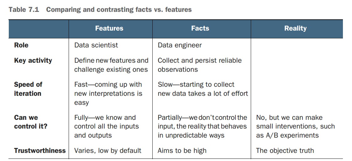
-
Facts:
- Direct, objective observations from reality (e.g., a user clicks "Play").
- Collected by data engineers with minimal interpretation.
- Stored in reliable fact tables for reuse across projects.
- Can be biased or noisy but represent raw events as-is.
-
Features:
- Interpretations or transformations of facts, crafted for use in models.
- Created by data scientists and iterated based on modeling results.
- Numerous valid features can be derived from the same fact.
- Tailored to the use case and modeling task.
Why is distinguishing facts from features practically important?
-
Divides responsibilities:
- Data engineers handle infrastructure and data integrity.
- Data scientists focus on experimentation and modeling logic.
-
Enables iteration:
- Reliable facts allow repeatable extraction of different feature sets.
- Supports fast prototyping and evaluation cycles.
-
Encourages modularity:
- Fact tables are centralized and reusable.
- Feature generation happens downstream in workflows (e.g., using
foreachand Python UDFs).
How do facts and features relate to workflow patterns in this chapter?
-
Fact storage:
- Data engineers maintain high-quality, centralized fact tables.
-
CTAS pattern:
- Data scientists extract project-specific views from fact tables using SQL.
-
MapReduce-style workflows:
- Feature extraction and transformation occur in parallel (e.g., using
foreachin Metaflow).
- Feature extraction and transformation occur in parallel (e.g., using
What are suggested tools and patterns for working with features?
- Start with a simple, baseline solution using native workflows (e.g., Metaflow, SQL, Python).
- Consider integrating feature stores, labeling services, or custom libraries as needs grow.
- Ensure:
- Easy access to facts
- Fast feature iteration
- Versioning support (e.g., via Metaflow) to maintain traceability of data and feature sets.
Miscellaneous Notes
- There is no one-size-fits-all solution for feature engineering.
- Different data types (e.g., tabular, audio, time series) require different approaches.
- Domain expertise plays a critical role in choosing and transforming the right features.
Encoding features
What is feature encoding, and why is separating it from modeling important?
- Feature encoding (or featurization) transforms raw data (facts) into features usable by models.
- Done through feature encoder functions, which can number in the dozens or hundreds per project.
- Separation of featurization from modeling:
- Ensures maintainability and offline-online consistency (same encoders used during training and inference).
- Allows versioning and repeatability of ML workflows.
Why is managing time in feature encoding important?
- Prevents data leakage in time-series/backtesting scenarios by enforcing correct train-test splits.
- Enables modeling strategies like:
- Backtesting using a historical cut-off point.
- Concept drift detection by tracking how target feature statistics evolve.
- A well-structured encoding pipeline should respect time boundaries and modeling context.
Why is Python-based feature encoding sometimes preferable to SQL?
- Faster iteration: Testing assumptions (e.g., 2% outlier thresholds) is easier in Python.
- Complex logic: Multivariate outlier filtering and random sampling are simpler and more concise in Python.
- Performance: Leveraging Apache Arrow and NumPy avoids conversion to pandas, keeping computation fast and memory-efficient.
What utility functions support flexible featurization?
def filter_outliers(table, clean_fields):
    import numpy
    valid = numpy.ones(table.num_rows, dtype='bool')
    for field in clean_fields:
        column = table[field].to_numpy()
        minval = numpy.percentile(column, 2)
        maxval = numpy.percentile(column, 98)
        valid &= (column > minval) & (column < maxval)
    return table.filter(valid)

def sample(table, p):
    import numpy
return table.filter(numpy.random.random(table.num_rows) < p)- Filters top/bottom 2% of values in selected fields.
- Uniformly samples rows with probability
p.
How is modeling and visualization handled?
def fit(features):
    from sklearn.linear_model import LinearRegression
    d = features['trip_distance'].reshape(-1, 1)
    model = LinearRegression().fit(d, features['total_amount'])
    return model

def visualize(model, features):
    import matplotlib.pyplot as plt
    from io import BytesIO
    import numpy
    maxval = max(features['trip_distance'])
    line = numpy.arange(0, maxval, maxval / 1000)
    pred = model.predict(line.reshape(-1, 1))
    plt.rcParams.update({'font.size': 22})
    plt.scatter(data=features,
                x='trip_distance',
                y='total_amount',
                alpha=0.01,
                linewidth=0.5)
    plt.plot(line, pred, linewidth=2, color='black')
    plt.xlabel('Distance')
    plt.ylabel('Amount')
    fig = plt.gcf()
    fig.set_size_inches(18, 10)
    buf = BytesIO()
    fig.savefig(buf)
return buf.getvalue()- Fits a linear regression model on distance vs. amount.
- Visualizes the scatterplot with a fitted regression line.
How does the TaxiRegressionFlow demonstrate feature encoding in a workflow?
from metaflow import FlowSpec, step, conda, Parameter, \
    S3, resources, project, Flow

URLS = ['s3://ursa-labs-taxi-data/2014/10/',
        's3://ursa-labs-taxi-data/2014/11/']
NUM_SHARDS = 4
FIELDS = ['trip_distance', 'total_amount']

@conda_base(python='3.8.10')
@project(name='taxi_nyc')
class TaxiRegressionFlow(FlowSpec):

    sample = Parameter('sample', default=0.1)
    use_ctas = Parameter('use_ctas_data', help='Use CTAS data', default=False)

    @step
    def start(self):
        if self.use_ctas:
            self.paths = Flow('TaxiETLFlow').latest_run.data.paths
        else:
            with S3() as s3:
                objs = s3.list_recursive(URLS)
                self.paths = [obj.url for obj in objs]

        print("Processing %d Parquet files" % len(self.paths))
        n = max(round(len(self.paths) / NUM_SHARDS), 1)
        self.shards = [self.paths[i*n:(i+1)*n] for i in range(NUM_SHARDS - 1)]
        self.shards.append(self.paths[(NUM_SHARDS - 1) * n:])
        self.next(self.preprocess_data, foreach='shards')

    @resources(memory=16000)
    @conda(libraries={'pyarrow': '5.0.0'})
    @step
    def preprocess_data(self):
        from table_utils import filter_outliers, sample
        self.shard = None
        with S3() as s3:
            from pyarrow.parquet import ParquetDataset
            if self.input:
                objs = s3.get_many(self.input)
                table = ParquetDataset([obj.path for obj in objs]).read()
                table = sample(filter_outliers(table, FIELDS), self.sample)
                self.shard = {field: table[field].to_numpy() for field in FIELDS}
        self.next(self.join)

    @resources(memory=8000)
    @conda(libraries={'numpy': '1.21.1'})
    @step
    def join(self, inputs):
        from numpy import concatenate
        self.features = {}
        for f in FIELDS:
            shards = [inp.shard[f] for inp in inputs if inp.shard]
            self.features[f] = concatenate(shards)
        self.next(self.regress)

    @resources(memory=8000)
    @conda(libraries={'numpy': '1.21.1',
                      'scikit-learn': '0.24.1',
                      'matplotlib': '3.4.3'})
    @step
    def regress(self):
        from taxi_model import fit, visualize
        self.model = fit(self.features)
        self.viz = visualize(self.model, self.features)
        self.next(self.end)

    @step
    def end(self):
        pass

if __name__ == '__main__':
TaxiRegressionFlow()- Supports CTAS-based or raw S3 data.
- Uses
foreachto parallelize preprocessing. - Filters and samples data shards.
- Aggregates feature arrays for model fitting.
- Trains and visualizes a regression model.
python taxi_regression.py --environment=conda run --use_ctas_data=True- Omit
--use_ctas_data=Trueto use raw data. - Run takes ~1–2 minutes depending on sample size and instance size.
What are the key lessons from this example?
- Demonstrates a flexible and performant feature pipeline using:
- Query engines for extraction (CTAS).
- Python for encoding (Arrow + NumPy).
- Scikit-learn for modeling.
- Encodes features using a MapReduce-style pattern with
foreachandjoin. - Model results and visualizations are versioned in Metaflow.
Miscellaneous Notes
- This example is on the flexibility-focused end of the spectrum; not all best practices (e.g., online-offline consistency) are enforced.
- In Chapter 9, the pipeline will be expanded with more robust and extensible feature engineering patterns.
- Starting with a flexible system helps rapid iteration. Rigid systems for correctness can be introduced later as needed.