ch6.using_neural_network
Ch 6. Using a neural network to fit the data
Artificial Neurons: The Building Blocks of Neural Networks
Neural networks are mathematical models designed to approximate complex functions through the composition of simpler functions. While inspired by neuroscience, modern artificial neural networks only loosely resemble biological neurons.
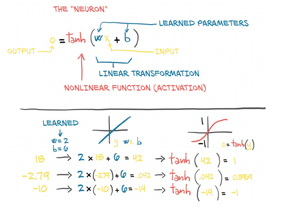
1. Structure of an Artificial Neuron
-
A neuron performs a linear transformation on its input, followed by a nonlinear activation function.
-
Mathematically:
$o = f(w \cdot x + b)$
where:
- $x$ = input (scalar or vector)
- $w$ = weight (scaling factor, scalar or matrix)
- $b$ = bias (offset, scalar or vector)
- $f$ = activation function (e.g.,
tanh,ReLU) - $o$ = output (transformed input)
✅ The activation function introduces non-linearity, allowing the network to approximate more complex relationships.
2. Layers of Neurons
- A single neuron is a fundamental unit, but neural networks consist of layers of neurons.
- A layer applies the same transformation to multiple inputs using matrix operations.
- If $x$ and $w$ are vectors/matrices, the equation extends to multiple neurons in parallel.
🚀 Key Idea: By stacking multiple layers, neural networks learn hierarchical representations of data.
3. Why Use Activation Functions?
Without an activation function:
- The neuron only applies a linear transformation, which is insufficient for complex problems.
- Activation functions introduce non-linearity, enabling networks to learn more expressive mappings.
Composing a Multilayer Network
-
A multilayer neural network consists of multiple layers where the output of one layer is the input to the next:
$x_1 = f(w_0 \cdot x + b_0)$
$x_2 = f(w_1 \cdot x_1 + b_1)$
$y = f(w_n \cdot x_n + b_n)$
-
Key Points:
- $w_0$ is a matrix, and $x$ is a vector—this allows multiple neurons to be processed in parallel.
- Each layer extracts features from the previous layer’s output, enabling deep networks to learn hierarchical representations.
Understanding the Error Function
- In linear models, the error function (loss) is typically convex, meaning it has a single minimum.
- Neural networks, however, have non-convex loss surfaces due to activation functions, leading to:
- Multiple local minima
- No single correct answer for parameters
- Parameter dependencies, meaning the network learns useful approximations rather than exact solutions.
⚠️ Why is the error function non-convex?
- Activation functions introduce non-linearity, enabling neural networks to approximate complex functions but also making optimization harder.
The Role of Activation Functions
- Activation functions serve two key purposes:
- Enable non-linearity: Allows different slopes at different values, enabling networks to approximate complex functions.
- Control output range: Ensures predictions remain within meaningful bounds.
Types of Activation Functions
| Activation | Equation | Output Range | Purpose |
|---|---|---|---|
| ReLU | $f(x) = \max(0, x)$ | $[0, \infty]$ | Avoids vanishing gradients, commonly used in hidden layers. |
| Sigmoid | $f(x) = \frac{1}{1 + e^{-x}}$ | $(0,1)$ | Good for probabilities but can cause vanishing gradients. |
| Tanh | $f(x) = \frac{e^x - e^{-x}}{e^x + e^{-x}}$ | $(-1,1)$ | Centered at 0, useful for outputs requiring both positive and negative values. |
| HardTanh | Caps values between $[-1,1]$ | $(-1,1)$ | Limits extreme outputs, preventing unstable training. |
Example: Dog Classification Using Tanh
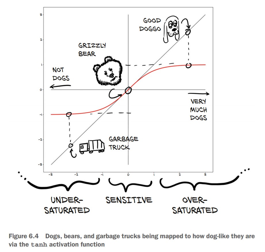
- Suppose we classify images as "good doggos" with a score from -1 (not a dog) to +1 (very much a dog).
- Some example outputs:
- Garbage truck → $-0.97$
- Bear → $-0.3$
- Golden retriever → $0.99$
import math

print(math.tanh(-2.2))  # Garbage truck → -0.97
print(math.tanh(0.1))   # Bear → 0.1
print(math.tanh(2.5)) # Golden Retriever → 0.99- Why does this work?
- Extreme values (garbage trucks, airplanes) are squashed close to -1.
- Small differences in middle values (e.g., bear vs. dog) affect classification.
- The activation range ensures meaningful outputs without extreme values.
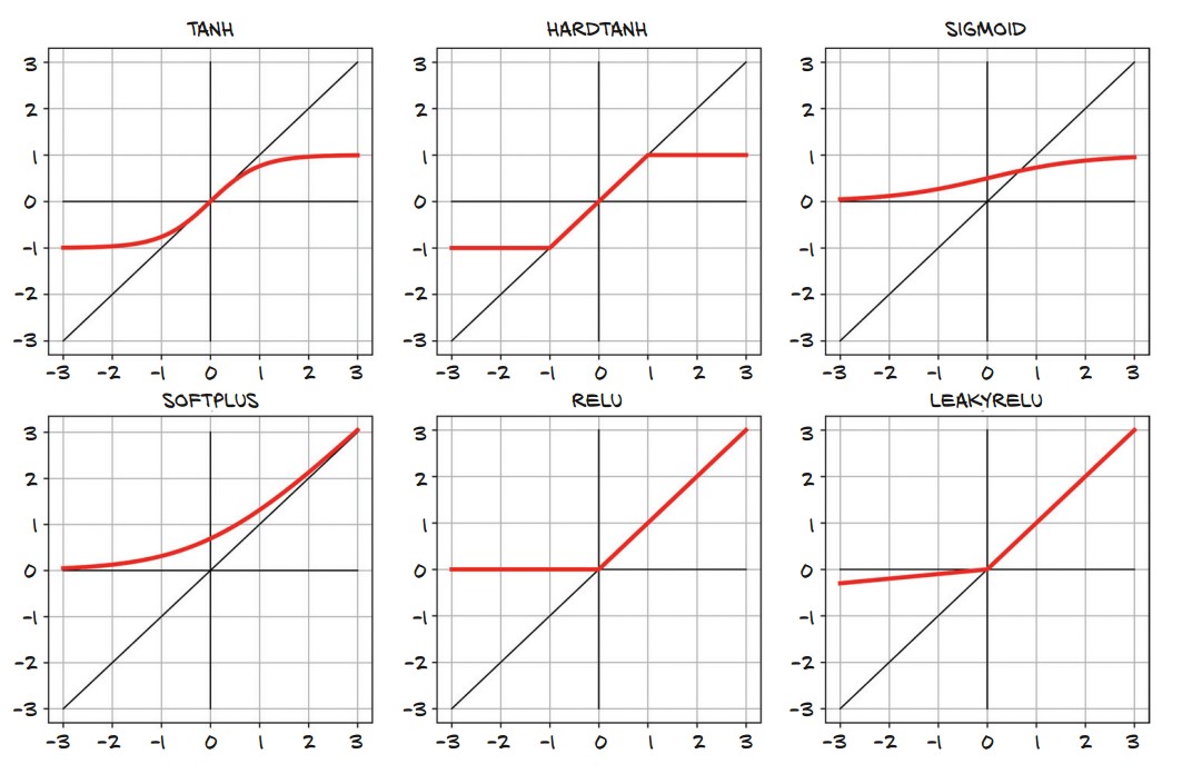
More Activation Functions
-
Types of Activation Functions:
- Smooth functions:
Tanh: Outputs values in $[-1, 1]$, useful for centered outputs.Softplus: A smooth approximation of ReLU.
- Piecewise linear functions:
Hardtanh: LikeTanhbut with hard saturation.ReLU(Rectified Linear Unit): Outputs $x$ if $x > 0$, otherwise 0.LeakyReLU: A variation of ReLU that allows small negative values instead of zero.
- Probability-based function:
Sigmoid: Outputs values in $(0,1)$, useful for probabilities.
- Smooth functions:
-
ReLU is widely used in deep learning due to its simplicity and effectiveness.
-
Sigmoid is rarely used except for probability-based outputs.
Choosing the Best Activation Function
-
Requirements for activation functions:
- Nonlinear: Without nonlinearity, the network collapses into a simple linear model.
- Differentiable: Needed for backpropagation.
- Sensitive range: Inputs should meaningfully affect outputs.
- Bounded (often): Keeps values in a defined range to prevent instability.
-
Backpropagation Considerations:
- Gradients are useful in the sensitive range but diminish in saturated areas.
- Certain neurons may become inactive if they reach the saturated region (e.g., "dead" ReLU neurons with outputs stuck at 0).
-
Key Takeaway: The right activation function depends on the task and how we want the network to behave.
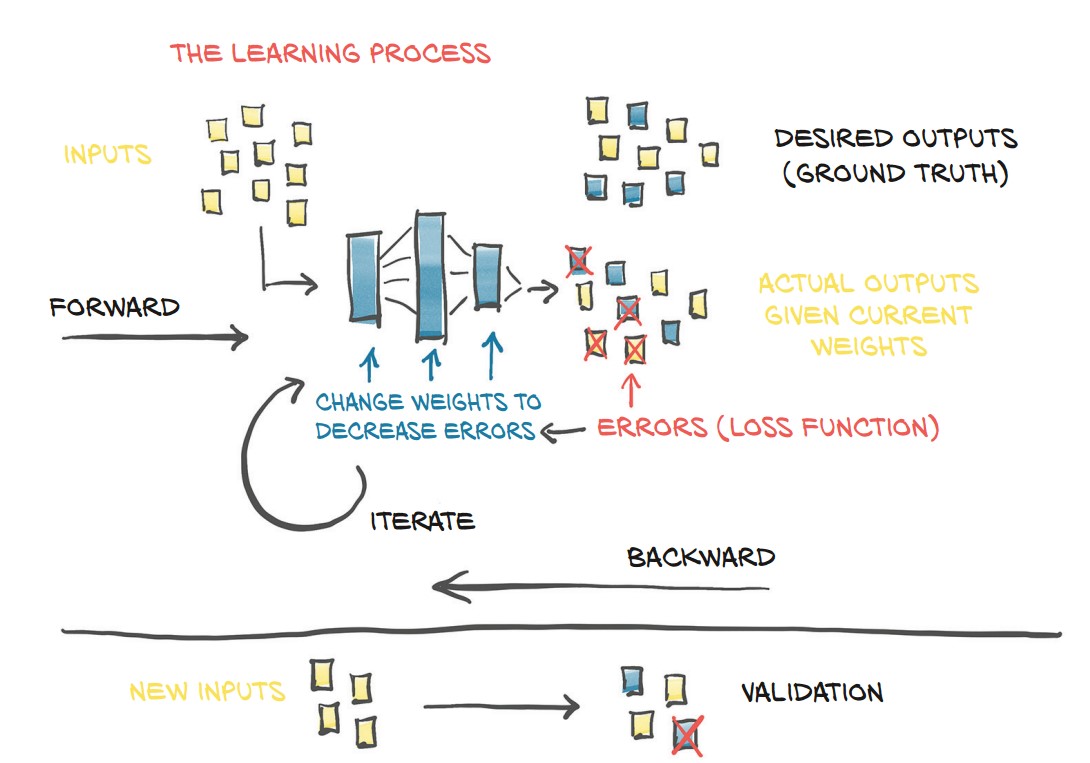
What Learning Means for a Neural Network
-
Neural networks approximate functions using stacks of linear transformations + activation functions.
-
Why deep learning is powerful:
- No need to assume an explicit function shape (e.g., quadratic or polynomial).
- Works well even with millions of parameters.
- Learns complex mappings between inputs and outputs.
-
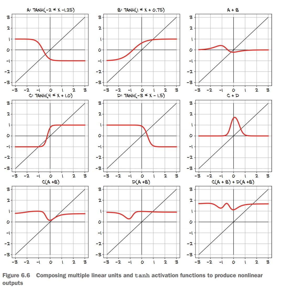
Example of how simple neurons combine:
- Single neurons (A, B, C, D) with different weights and biases create nonlinear functions.
- Adding neurons together (A+B, C+D) starts forming complex shapes.
- Stacking neurons in layers (e.g., C(A+B) + D(A+B)) results in highly flexible function approximations.
- Final insight:
- Traditional modeling: Requires an explicit formula.
- Neural networks: Learn patterns without needing an explicit equation.
- Tradeoff: We lose interpretability but gain the ability to solve complex problems.
📌 Key Takeaway: Deep learning trades explicit modeling for flexibility, making it effective for problems where traditional equations fail. 🚀
The PyTorch nn Module
- Purpose: Provides building blocks (modules) for constructing neural networks.
- Key Concept: A module is a Python class that inherits from
nn.Module. It can contain:- Parameters (learnable tensors like weights & biases).
- Submodules (nested layers inside a model).
Using __call__ Rather Than forward
- Calling a module (e.g.,
linear_model(input)) calls itsforward()method. - Do not call
forward()directly because:__call__also handles hooks and other PyTorch internals.
Example:
import torch.nn as nn

linear_model = nn.Linear(1, 1)  # One input feature, one output feature
output = linear_model(torch.tensor([[0.5], [14.0]]))
print(output)  # Output tensor with gradient tracking
Returning to the Linear Model
-
Defining a Linear Layer:
linear_model = nn.Linear(1, 1) # One input, one output -
Checking Initial Weights & Bias:
print(linear_model.weight)  # Randomly initialized weight
print(linear_model.bias)    # Randomly initialized bias
Batching Inputs
-
Why Batch Inputs?
- Efficiently utilizes GPUs (parallel computation).
- Some models rely on batch statistics.
-
Batch Format:
- Input tensors should be B × Nin (batch size × number of features).
- Output tensors will be B × Nout (batch size × output features).
-
Reshaping Inputs:
t_u = torch.tensor([35.7, 55.9, 58.2]).unsqueeze(1)  # Shape: (B, 1)
print(t_u.shape)  # torch.Size([3, 1])
Updating the Training Code
-
Define Model & Optimizer:
linear_model = nn.Linear(1, 1) optimizer = torch.optim.SGD(linear_model.parameters(), lr=1e-2) -
Using PyTorch's Built-in Loss Function:
loss_fn = nn.MSELoss() # Mean Squared Error loss -
Updated Training Loop:
def training_loop(n_epochs, optimizer, model, loss_fn, t_u_train, t_u_val, t_c_train, t_c_val): for epoch in range(1, n_epochs + 1): t_p_train = model(t_u_train) loss_train = loss_fn(t_p_train, t_c_train) with torch.no_grad(): # Disable gradient tracking for validation t_p_val = model(t_u_val) loss_val = loss_fn(t_p_val, t_c_val) optimizer.zero_grad() loss_train.backward() optimizer.step() if epoch == 1 or epoch % 1000 == 0: print(f"Epoch {epoch}, Training loss {loss_train.item():.4f}, Validation loss {loss_val.item():.4f}") return model -
Run Training:
linear_model = nn.Linear(1, 1)
optimizer = torch.optim.SGD(linear_model.parameters(), lr=1e-2)

training_loop(
    n_epochs=3000,
    optimizer=optimizer,
    model=linear_model,
    loss_fn=nn.MSELoss(),
    t_u_train=t_un_train,
    t_u_val=t_un_val,
    t_c_train=t_c_train,
    t_c_val=t_c_val
)

print(linear_model.weight)
print(linear_model.bias)
Results
- Training converges similarly to our manual implementation.
- Output example:
Epoch 1, Training loss 134.9599, Validation loss 183.1707
Epoch 1000, Training loss 4.8053, Validation loss 4.7307
Epoch 2000, Training loss 3.0285, Validation loss 3.0889
Epoch 3000, Training loss 2.8569, Validation loss 3.9105
tensor([[5.4319]], requires_grad=True)
tensor([-17.9693], requires_grad=True)
Finally, a Neural Network
- Goal: Replace the simple linear model with a neural network.
- Key Idea: Introduce a hidden layer with a non-linear activation function (
Tanh).
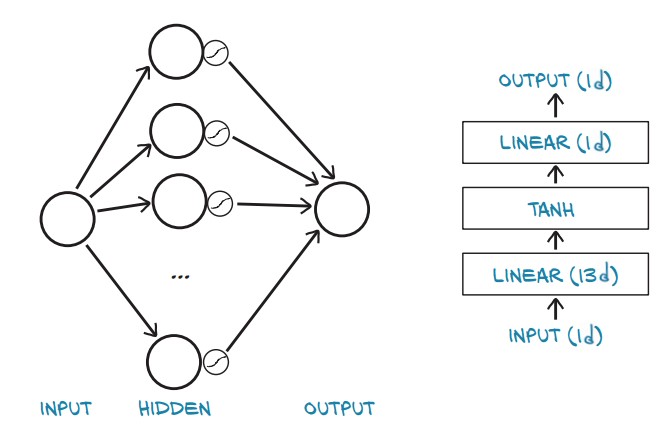
- The model consists of:
- First Linear Layer (
nn.Linear(1, 13)) – Expands from 1 input feature to 13 hidden units. - Activation (
nn.Tanh()) – Introduces non-linearity. - Second Linear Layer (
nn.Linear(13, 1)) – Reduces hidden units to 1 output.
- First Linear Layer (
Using nn.Sequential to Define the Model:
import torch.nn as nn

seq_model = nn.Sequential(
    nn.Linear(1, 13),  # Input layer to hidden layer (1 → 13)
    nn.Tanh(),         # Activation function
    nn.Linear(13, 1)   # Hidden layer to output (13 → 1)
)

print(seq_model)
Output:
Sequential(
  (0): Linear(in_features=1, out_features=13, bias=True)
  (1): Tanh()
  (2): Linear(in_features=13, out_features=1, bias=True)
)
Inspecting Model Parameters
- The model contains multiple trainable parameters:
- Weights and Biases for both Linear Layers.
[param.shape for param in seq_model.parameters()][torch.Size([13, 1]), torch.Size([13]), torch.Size([1, 13]), torch.Size([1])]- First
Linear(1, 13):weight:[13, 1]bias:[13]
- Second
Linear(13, 1):weight:[1, 13]bias:[1]
Viewing Parameter Names:
for name, param in seq_model.named_parameters():
    print(name, param.shape)
Output:
0.weight torch.Size([13, 1])
0.bias torch.Size([13])
2.weight torch.Size([1, 13])
2.bias torch.Size([1])
Using OrderedDict for More Descriptive Naming:
from collections import OrderedDict

seq_model = nn.Sequential(OrderedDict([
    ('hidden_linear', nn.Linear(1, 8)),
    ('hidden_activation', nn.Tanh()),
    ('output_linear', nn.Linear(8, 1))
]))- Now, parameter names are more descriptive:
for name, param in seq_model.named_parameters():
    print(name, param.shape)
Output:
hidden_linear.weight torch.Size([8, 1])
hidden_linear.bias torch.Size([8])
output_linear.weight torch.Size([1, 8])
output_linear.bias torch.Size([1])
Training the Neural Network
- Update Training Loop:
import torch.optim as optim

optimizer = optim.SGD(seq_model.parameters(), lr=1e-3)

training_loop(
    n_epochs=5000,
    optimizer=optimizer,
    model=seq_model,
    loss_fn=nn.MSELoss(),
    t_u_train=t_un_train,
    t_u_val=t_un_val,
    t_c_train=t_c_train,
    t_c_val=t_c_val
)

print('output', seq_model(t_un_val))
print('answer', t_c_val)
print('hidden', seq_model.hidden_linear.weight.grad)
Output (Sample Epochs & Predictions):
Epoch 1, Training loss 182.9724, Validation loss 231.8708
Epoch 1000, Training loss 6.6642, Validation loss 3.7330
Epoch 2000, Training loss 5.1502, Validation loss 0.1406
Epoch 3000, Training loss 2.9653, Validation loss 1.0005
Epoch 4000, Training loss 2.2839, Validation loss 1.6580
Epoch 5000, Training loss 2.1141, Validation loss 2.0215
output tensor([[-1.9930],
               [20.8729]], grad_fn=<AddmmBackward>)
answer tensor([[-4.],
               [21.]])
hidden tensor([[ 0.0272], [ 0.0139], [ 0.1692], [ 0.1735],
               [-0.1697], [ 0.1455], [-0.0136], [-0.0554]])
Comparing Neural Network vs. Linear Model
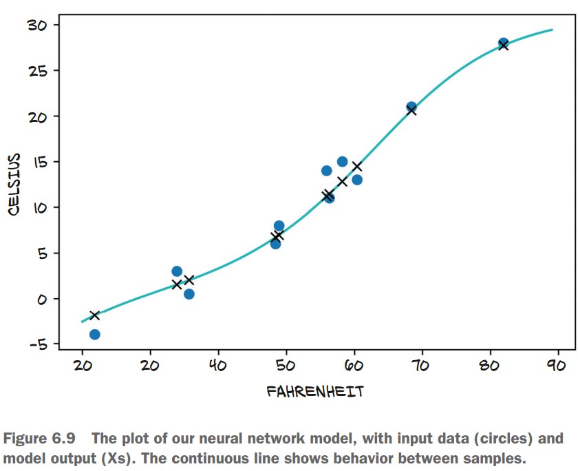
- Plot Predictions:
import matplotlib.pyplot as plt

t_range = torch.arange(20., 90.).unsqueeze(1)

fig = plt.figure(dpi=600)
plt.xlabel("Fahrenheit")
plt.ylabel("Celsius")
plt.plot(t_u.numpy(), t_c.numpy(), 'o')  # Original data points
plt.plot(t_range.numpy(), seq_model(0.1 * t_range).detach().numpy(), 'c-')  # NN Predictions
plt.plot(t_u.numpy(), seq_model(0.1 * t_u).detach().numpy(), 'kx') # Predictions at training points- Observations:
- The neural network overfits the data by following noise too closely.
- The simple linear model generalizes better for this problem.