ch4.data_representation
Ch 4. Real-world data representation using tensors
Working with Images in PyTorch
To process image data in PyTorch, we need to:
- Load an image file into a tensor.
- Change its layout to match PyTorch’s expected format (C × H × W).
- Normalize pixel values for efficient neural network training.
1. Loading an Image File
Images come in various formats (PNG, JPEG, etc.), and Python provides multiple libraries to load them. Here, we use imageio for its flexibility.
Reading an Image as a NumPy Array
import imageio

img_arr = imageio.imread('../data/p1ch4/image-dog/bobby.jpg')
print(img_arr.shape)  # Output: (720, 1280, 3) -> (Height, Width, Channels)
✅ The image is stored as a NumPy array with dimensions H × W × C (Height × Width × Channels).
✅ PyTorch requires the format C × H × W for deep learning models.
2. Changing the Layout (H × W × C → C × H × W)
Use torch.permute() to rearrange the dimensions.
import torch

img = torch.from_numpy(img_arr)  # Convert NumPy array to PyTorch tensor
img = img.permute(2, 0, 1)  # Reorder to (Channels, Height, Width)
print(img.shape)  # Output: (3, 720, 1280)
✅ permute(2, 0, 1) moves the third dimension (C) to the first position.
✅ This operation does not copy the data—it's an efficient, view-based transformation.
3. Processing a Batch of Images
To train a model, we process multiple images in a batch. A batch tensor should have the shape N × C × H × W (Batch size, Channels, Height, Width).
Preallocating a Batch Tensor
batch_size = 3
batch = torch.zeros(batch_size, 3, 256, 256, dtype=torch.uint8)  # Preallocated batch tensor
Loading Multiple Images into the Batch
import os

data_dir = '../data/p1ch4/image-cats/'
filenames = [name for name in os.listdir(data_dir) if name.endswith('.png')]

for i, filename in enumerate(filenames):
    img_arr = imageio.imread(os.path.join(data_dir, filename))  # Read image
    img_t = torch.from_numpy(img_arr)  # Convert to tensor
    img_t = img_t.permute(2, 0, 1)  # Convert to C × H × W format
    img_t = img_t[:3]  # Keep only RGB channels if an alpha channel is present
    batch[i] = img_t  # Store in batch tensor
✅ The batch now holds 3 RGB images of size 256×256 pixels.
4. Normalizing the Data
Neural networks work best when input values are scaled to a small range (e.g., 0–1 or -1 to 1).
Option 1: Normalize to [0, 1]
batch = batch.float()  # Convert to float
batch /= 255.0  # Scale values between 0 and 1
✅ Converts uint8 (0–255) pixel values to floating-point (0.0–1.0).
Option 2: Standardization (Zero Mean, Unit Variance)
n_channels = batch.shape[1]  # Get number of channels (C)

for c in range(n_channels):
    mean = torch.mean(batch[:, c])  # Compute mean for each channel
    std = torch.std(batch[:, c])  # Compute standard deviation
    batch[:, c] = (batch[:, c] - mean) / std  # Normalize
✅ Ensures the dataset has zero mean and unit variance, improving stability during training.
✅ Best practice: Compute mean and std on the entire dataset (not just one batch).
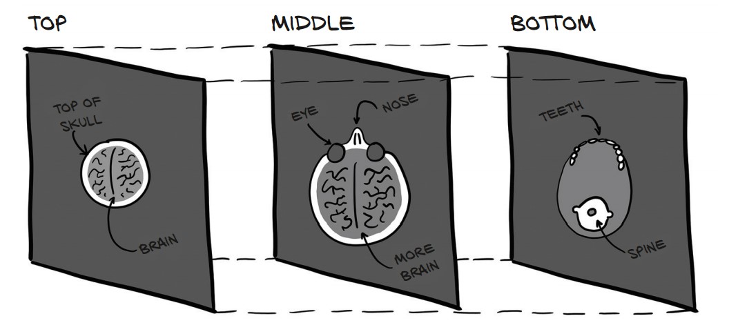
Working with 3D Volumetric Data (CT Scans) in PyTorch
CT scans provide 3D medical imaging data, where each slice represents a cross-section of the body. In PyTorch, we represent volumetric data as a 5D tensor with dimensions:
N × C × D × H × W → (Batch, Channels, Depth, Height, Width)
1. Loading a CT Scan
CT scan data is often stored in DICOM format (Digital Imaging and Communications in Medicine). The imageio library provides volread() to read a full scan from a directory.
Read a CT Scan from a Directory
import imageio

dir_path = "../data/p1ch4/volumetric-dicom/2-LUNG 3.0 B70f-04083"
vol_arr = imageio.volread(dir_path, 'DICOM')
print(vol_arr.shape)  # Output: (99, 512, 512)
✅ 99 slices of 512 × 512 pixels
✅ No color channels—this is grayscale intensity data.
2. Converting to a PyTorch Tensor
PyTorch expects an explicit channel dimension. Since the CT scan is grayscale, we add a dummy channel (size 1) using torch.unsqueeze().
Convert and Reshape Data
import torch

vol = torch.from_numpy(vol_arr).float()  # Convert NumPy array to PyTorch tensor
vol = torch.unsqueeze(vol, 0)  # Add a channel dimension
print(vol.shape)  # Output: torch.Size([1, 99, 512, 512])
✅ Shape is now [1, Depth, Height, Width] (C × D × H × W)
✅ The extra dimension is crucial for deep learning models.
3. Preparing a Batch of 3D CT Scans
To process multiple CT scans, we stack them along the batch dimension (N).
Building a Batch Tensor (N × C × D × H × W)
batch_size = 5  # Example batch size
batch = torch.zeros(batch_size, 1, 99, 512, 512)  # Preallocate batch tensor

# Load multiple CT scans into the batch
for i in range(batch_size):
    vol_arr = imageio.volread(f"../data/p1ch4/ct_scan_{i}/", 'DICOM')
    vol_t = torch.from_numpy(vol_arr).float().unsqueeze(0)  # Add channel dimension
    batch[i] = vol_t  # Store in batch tensor

print(batch.shape)  # Output: torch.Size([5, 1, 99, 512, 512])
4. Normalizing CT Scan Data
CT scans use Hounsfield units (HU) to measure tissue density. Neural networks train better when input values are normalized.
# Normalize to `[0, 1]`
batch = batch / batch.max()

# Normalize to Zero Mean, Unit Variance
mean = torch.mean(batch)
std = torch.std(batch)
batch = (batch - mean) / std
✅ Improves model performance and stability.
Working with Tabular Data in PyTorch
Tabular data consists of rows (samples) and columns (features). PyTorch requires tabular data to be converted into numerical tensors for processing.
1. Loading a Real-World Dataset (Wine Quality)
The Wine Quality Dataset contains chemical properties of wine samples and their quality scores (0–10).
Load the CSV File
import numpy as np

wine_path = "../data/p1ch4/tabular-wine/winequality-white.csv"
wineq_numpy = np.loadtxt(wine_path, dtype=np.float32, delimiter=";", skiprows=1)
print(wineq_numpy.shape)  # Output: (4898, 12) -> 4898 samples, 12 columns
✅ First 11 columns = Chemical properties
✅ Last column = Quality score (0-10)
2. Converting Data to PyTorch Tensors
import torch

wineq = torch.from_numpy(wineq_numpy)
print(wineq.shape, wineq.dtype)  # Output: torch.Size([4898, 12]), torch.float32
✅ Converted NumPy array to PyTorch tensor
3. Separating Features and Target
The last column is the target (quality score), and the first 11 columns are features.
Extract Features (X) and Target (y)
data = wineq[:, :-1]  # Features (first 11 columns)
target = wineq[:, -1]  # Target (last column)
print(data.shape, target.shape)  # Output: torch.Size([4898, 11]), torch.Size([4898])
✅ data (X) → Features (11 chemical properties)
✅ target (y) → Quality score
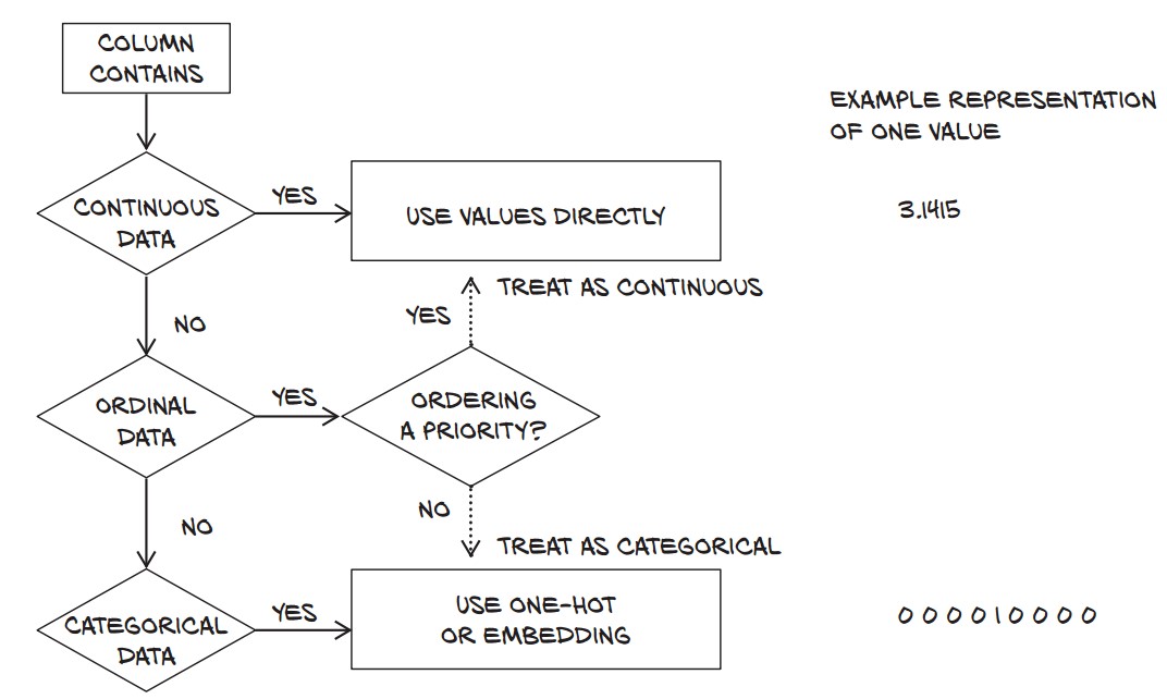
4. Understanding Data Types in Machine Learning
Tabular data can have three types of numerical values:
| Type | Example | Properties |
|---|---|---|
| Continuous | pH, Alcohol | Ordered, meaningful differences |
| Ordinal | Small (1), Large (3) | Ordered, but no fixed scale |
| Categorical | Red (0), White (1) | No ordering, just labels |
5. Handling Target Variable
The quality score (0-10) can be treated as:
- Regression → Keep as a continuous value (
float32) - Classification → Convert to an integer (
long)
Convert Target to Integer for Classification
target = target.long()
print(target[:5])  # Output: tensor([6, 6, 6, 6, 6])
✅ Now ready for classification models!
6. One-Hot Encoding for Categorical Data
- When when dealing with classification problems, one-hot encoding is often used to represent categorical targets efficiently.
- One-hot encoding creates binary vectors for categorical labels.
- In classification tasks, the target variable is often categorical. The wine quality scores range from 0 to 9 (discrete values), but machine learning models prefer numerical representations.
- One-hot encoding converts a categorical variable into a binary matrix where:
- Each class label is represented as a vector of all zeros except for a
1at the index of the class.
For example:
| Target Value | One-Hot Encoded |
|---|---|
| 3 | [0, 0, 0, 1, 0, 0, 0, 0, 0, 0] |
| 5 | [0, 0, 0, 0, 0, 1, 0, 0, 0, 0] |
| 8 | [0, 0, 0, 0, 0, 0, 0, 0, 1, 0] |
Convert Quality Score to One-Hot Encoding
target_onehot = torch.zeros(target.shape[0], 10)  # Create a 4898 × 10 tensor of zeros
target_onehot.scatter_(1, target.unsqueeze(1), 1.0) # Set 1 at index of target score-
Create a Zero Tensor (
torch.zeros(target.shape[0], 10))- Generates a tensor of shape
(4898, 10)initialized with zeros. - Each row corresponds to a wine sample.
- Each column corresponds to one of the 10 possible target values (0-9).
- Generates a tensor of shape
-
Use
.scatter_()to Place1.0at the Correct Indextarget.unsqueeze(1)Reshapestargetfrom(4898,)to(4898, 1)scatter_()expects a column vector of indices.
scatter_(dim, index, value)dim=1: Scatter values along columns (i.e., across the one-hot dimension).index=target.unsqueeze(1): Specifies which column in each row should be set to1.0.value=1.0: Assigns 1.0 to the correct position.
Example of scatter_() in Action
Assume target contains:
target = torch.tensor([3, 5, 8])The one-hot encoding process would look like:
target_onehot = torch.zeros(3, 10)  # Creates a 3 × 10 zero matrix
target_onehot.scatter_(1, target.unsqueeze(1), 1.0)
print(target_onehot)
Output:
tensor([[0., 0., 0., 1., 0., 0., 0., 0., 0., 0.],  # target = 3
        [0., 0., 0., 0., 0., 1., 0., 0., 0., 0.],  # target = 5
        [0., 0., 0., 0., 0., 0., 0., 0., 1., 0.]]) # target = 8
Why Do We Use One-Hot Encoding?
- Required for Neural Networks
- Most classification models (e.g., neural networks) expect labels to be one-hot encoded rather than raw integer values.
- Example: Softmax activation function expects inputs in one-hot format.
- Better for Multi-Class Classification
- If the target has multiple classes, one-hot encoding allows models to treat them as independent categories.
- Example: Instead of treating
3,5, and8as numbers, the model learns them as distinct classes.
- Allows for More Flexible Loss Functions
- Cross-Entropy Loss (
torch.nn.CrossEntropyLoss):- Works with class indices (not one-hot) →
targetcan remain as a single integer.
- Works with class indices (not one-hot) →
- Binary Cross-Entropy (
torch.nn.BCELoss):- Requires one-hot encoding if applied to multi-class problems.
Normalizing Data
Neural networks perform better when input data is normalized (mean = 0, variance = 1).
data_mean = torch.mean(data, dim=0)
data_var = torch.var(data, dim=0)dim=0→ Compute along columns (features)data_mean→ Column-wise meandata_var→ Column-wise variance
data_normalized = (data - data_mean) / torch.sqrt(data_var)Filtering Based on Quality Score
To analyze wine quality categories, we split the data into:
bad_data = data[target <= 3]
mid_data = data[(target > 3) & (target < 7)]
good_data = data[target >= 7]
Analyzing Differences Between Wine Groups
bad_mean = torch.mean(bad_data, dim=0)
mid_mean = torch.mean(mid_data, dim=0)
good_mean = torch.mean(good_data, dim=0)

for i, args in enumerate(zip(col_list, bad_mean, mid_mean, good_mean)):
    print('{:2} {:20} {:6.2f} {:6.2f} {:6.2f}'.format(i, *args))
Findings:
- Bad wines have higher total sulfur dioxide (170.6) than good wines (125.2).
- Alcohol content is higher in good wines (11.4 vs. 10.3).
- Acidity is slightly lower in good wines.
✅ Feature selection can help predict quality! 🎯
Using a Threshold to Predict Good Wines
Let’s predict high-quality wines based on total sulfur dioxide.
total_sulfur_threshold = 141.83
total_sulfur_data = data[:, 6]  # Column index for total sulfur dioxide
predicted_indexes = torch.lt(total_sulfur_data, total_sulfur_threshold)
✅ Predicted "good wines" = 2,727 samples
Compare Predictions to Actual Data
actual_indexes = target > 5  # Wines rated >5 are good
print(actual_indexes.sum())  # Output: 3,258 (actual good wines)
✅ Actual "good wines" = 3,258 samples (more than predicted)
Evaluating Prediction Accuracy
We check how well our threshold works using logical AND (&).
Count Correct Predictions
n_matches = torch.sum(actual_indexes & predicted_indexes).item()
n_predicted = torch.sum(predicted_indexes).item()
n_actual = torch.sum(actual_indexes).item()

print(n_matches, n_matches / n_predicted, n_matches / n_actual)- 2,018 wines correctly classified 🎯
- Precision: 74% (Good wine predictions were correct 74% of the time)
- Recall: 61% (Only 61% of actual good wines were found)
✅ Thresholding is simple but inaccurate.
✅ A neural network can model complex relationships better. 🚀
Working with Time Series in PyTorch
Loading and Preparing the Dataset
The dataset records hourly bike rentals with weather and seasonal data. Each row represents an hour.
bikes_numpy = np.loadtxt(
    "../data/p1ch4/bike-sharing-dataset/hour-fixed.csv",
    dtype=np.float32,
    delimiter=",",
    skiprows=1,
    converters={1: lambda x: float(x[8:10])}  # Extract day from datetime
)
bikes = torch.from_numpy(bikes_numpy)
print(bikes.shape)  # (17520, 17)
✅ Shape: (17,520 rows × 17 columns) → Rows represent hours, columns contain features.
Each day has 24 hours → Reshape dataset into days × hours × features.
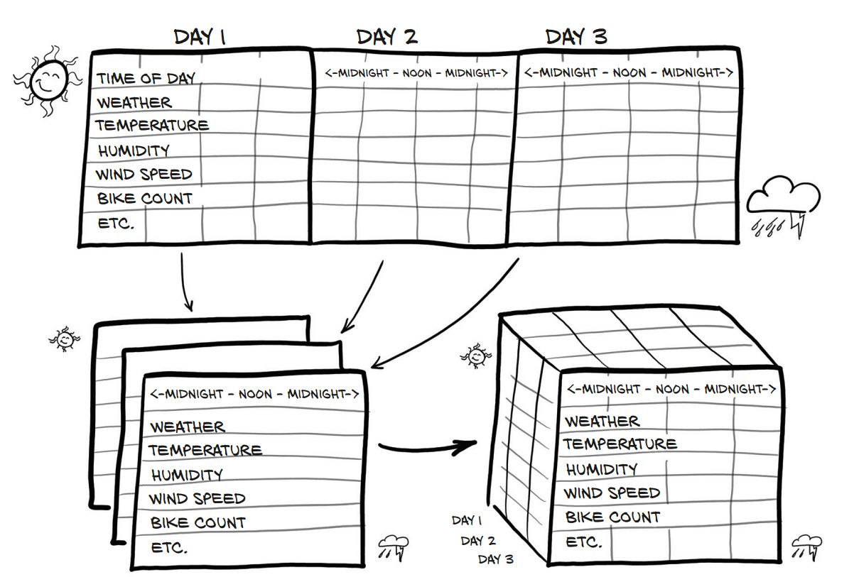
Reshape to (Days, Hours, Features)
daily_bikes = bikes.view(-1, 24, bikes.shape[1])
print(daily_bikes.shape)  # (730 days, 24 hours, 17 features)
.view(-1, 24, 17)→ Groups data by days (automatic computation using-1).- Stride Analysis (
daily_bikes.stride())print(daily_bikes.stride()) # (408, 17, 1)- Day-to-Day Move → 408 elements (24 × 17).
- Hour-to-Hour Move → 17 elements (all features for an hour).
- Feature-to-Feature Move → 1 element (within an hour).
Rearrange for PyTorch (N × C × L)
daily_bikes = daily_bikes.transpose(1, 2)
print(daily_bikes.shape)  # (730, 17, 24)
✅ Final shape: (730 days, 17 features, 24 hours) → Ready for training!
Handling Ordinal and Categorical Variables
One-Hot Encoding of "Weather Situation"
first_day = bikes[:24].long()  # First 24 rows (1 day)
weather_onehot = torch.zeros(first_day.shape[0], 4)  # 4 categories

weather_onehot.scatter_(
    dim=1,
    index=first_day[:, 9].unsqueeze(1).long() - 1,  # Adjust for 0-based index
    value=1.0
)
print(weather_onehot[:5])  # First 5 rows
✅ One-hot encoding expands categorical variable into binary columns.
Concatenating One-Hot Data to Original Data
bikes_onehot = torch.cat((bikes[:24], weather_onehot), dim=1)
print(bikes_onehot.shape)  # (24, 21) → 4 new one-hot columns
✅ New feature space! Adds 4 weather situation columns.
Normalizing Continuous Data
Rescaling weather situation (0-1 range)
daily_bikes[:, 9, :] = (daily_bikes[:, 9, :] - 1.0) / 3.0✅ Good practice for neural networks.
Rescale Temperature to [0,1]
temp = daily_bikes[:, 10, :]
temp_min, temp_max = temp.min(), temp.max()
daily_bikes[:, 10, :] = (temp - temp_min) / (temp_max - temp_min)
✅ Min-max normalization improves training.
Standardize Temperature (Zero Mean, Unit Variance)
temp_mean, temp_std = temp.mean(), temp.std()
daily_bikes[:, 10, :] = (temp - temp_mean) / temp_std
✅ Standardization helps gradient-based optimization.
Representing Text in PyTorch
1. Converting Text to Numbers
- Deep learning models process text numerically using one-hot encoding or embeddings.
- Text can be represented at character-level or word-level.
Load Text Data (Jane Austen's Pride and Prejudice)
with open('../data/p1ch4/jane-austen/1342-0.txt', encoding='utf8') as f:
    text = f.read()
One-Hot Encoding Characters
Each character is represented as a vector with zeros everywhere except for one at the character’s index.
lines = text.split('\n')  # Split text into lines
line = lines[200]  # Pick an example line
print(line)
# Output: “Impossible, Mr. Bennet, impossible, when I am not acquainted with him”

letter_t = torch.zeros(len(line), 128)  # 128 possible ASCII characters

for i, letter in enumerate(line.lower().strip()):
    letter_index = ord(letter) if ord(letter) < 128 else 0  # Ignore non-ASCII
    letter_t[i][letter_index] = 1
✅ Each row in letter_t is a one-hot encoded character.
One-Hot Encoding Words
- Word-based encoding reduces sequence length but increases vocabulary size.
- Large vocabulary = huge one-hot vectors → inefficient.
Clean Text and Tokenize
def clean_words(input_str):
    punctuation = '.,;:"!?”“_-'
    word_list = input_str.lower().replace('\n', ' ').split()
    word_list = [word.strip(punctuation) for word in word_list]
    return word_list

words_in_line = clean_words(line)
print(words_in_line)
# Output: ['impossible', 'mr', 'bennet', 'impossible', 'when', 'i', 'am', 'not', 'acquainted', 'with', 'him']
✅ Text is now split into clean words.
Create Word-to-Index Mapping
word_list = sorted(set(clean_words(text)))  # Get unique words
word2index_dict = {word: i for i, word in enumerate(word_list)}
print(len(word2index_dict), word2index_dict['impossible'])
# Output: (7261, 3394)
✅ Created dictionary mapping words to unique indices.
One-Hot Encode Words
word_t = torch.zeros(len(words_in_line), len(word2index_dict))  # One-hot tensor

for i, word in enumerate(words_in_line):
    word_index = word2index_dict[word]
    word_t[i][word_index] = 1

print(word_t.shape)  # (11, 7261) → 11 words, 7261 vocabulary size
✅ Each row in word_t is a one-hot encoded word.
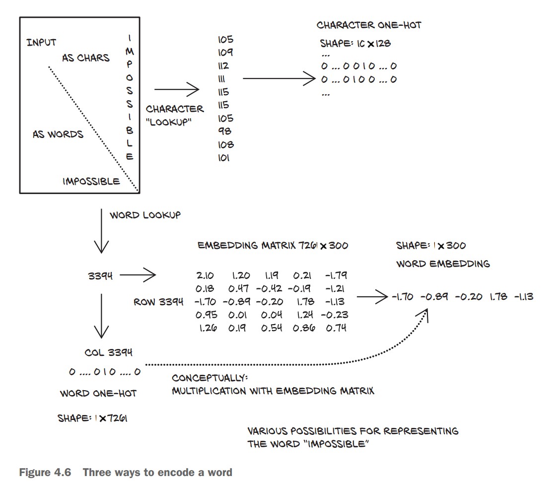
Using Text Embeddings
One-hot encoding represents each word as a binary vector of size equal to the vocabulary. While this works for small datasets, it becomes impractical when dealing with large vocabularies, such as in natural language processing (NLP).
Problems with One-Hot Encoding in NLP
-
High-Dimensionality (Curse of Dimensionality)
- If a vocabulary contains 100,000 words, then each word is represented as a 100,000-dimensional vector.
- Most elements in the vector are
0(sparse representation). - Consumes a lot of memory and slows down computations.
-
No Semantic Relationships Between Words
- One-hot encoding treats words as completely independent entities.
- Example:
"apple" → [0, 0, 0, 1, 0, 0, 0, ...] (100,000 elements) "banana" → [0, 1, 0, 0, 0, 0, 0, ...] (100,000 elements) - There is no numerical similarity between related words (e.g., "apple" and "banana").
- The model has no way to understand word relationships beyond explicit training.
How Embeddings Solve This Problem
Instead of using sparse one-hot vectors, embeddings map words to dense, lower-dimensional vectors where similar words have similar representations.
What are Word Embeddings?
- Each word is mapped to a fixed-size dense vector.
- Instead of a 100,000-dimensional sparse vector, a word might be represented as a 100-dimensional dense vector.
- These embeddings are learned during training and capture semantic meaning.
Example: Word Embeddings for "apple" and "banana"
Instead of:
"apple" → [0, 0, 0, 1, 0, 0, 0, ...] (100,000 dimensions)
"banana" → [0, 1, 0, 0, 0, 0, 0, ...] (100,000 dimensions)
We get:
"apple"  → [ 0.12, -0.55,  0.89, ...] (100 floats)
"banana" → [ 0.10, -0.51, 0.85, ...] (similar vector)- Only 100 dimensions instead of 100,000 (memory-efficient).
- Words with similar meanings have similar vector values.
Key Benefits of Word Embeddings
-
✅ Dimensionality Reduction
- Instead of a massive sparse vector, each word is represented by a compact vector (e.g., 100 dimensions instead of 100,000).
- Faster computations and less memory usage.
-
✅ Capturing Word Similarities
- Word embeddings preserve semantic relationships.
- Example: The cosine similarity between "apple" and "banana" will be higher than between "apple" and "table".
-
✅ Context-Aware Representations
- Advanced embeddings (like Word2Vec, GloVe, BERT) capture word meanings based on context.
- Example: The word "bank" has different meanings in:
- "I deposited money at the bank."
- "I sat by the bank of the river."
- Contextual embeddings (like BERT) assign different vectors based on meaning.
How Are Embeddings Used in PyTorch?
- PyTorch provides a built-in embedding layer:
torch.nn.Embedding
import torch
import torch.nn as nn

# Define an embedding layer (for 100,000 words, each represented by a 100-d vector)
embedding = nn.Embedding(num_embeddings=100000, embedding_dim=100)

# Example: Convert word indices to embeddings
word_index = torch.tensor([5, 123, 99999])  # Sample word indices
word_vectors = embedding(word_index)

print(word_vectors.shape) # Output: torch.Size([3, 100]) (3 words, each with 100-d vector)- Each word index (an integer) is mapped to a 100-dimensional vector.
- This is learned during training and adjusts based on the dataset.